Last updated: 2020-07-14

Checks: 7 0

Knit directory: QGT-Columbia-HKI-repo/

This reproducible R Markdown analysis was created with workflowr (version 1.6.2). The Checks tab describes the reproducibility checks that were applied when the results were created. The Past versions tab lists the development history.

R Markdown file: up-to-date

Great! Since the R Markdown file has been committed to the Git repository, you know the exact version of the code that produced these results.

Environment: empty

Great job! The global environment was empty. Objects defined in the global environment can affect the analysis in your R Markdown file in unknown ways. For reproduciblity it’s best to always run the code in an empty environment.

Seed: set.seed(20200603)

The command set.seed(20200603) was run prior to running the code in the R Markdown file. Setting a seed ensures that any results that rely on randomness, e.g. subsampling or permutations, are reproducible.

Session information: recorded

Great job! Recording the operating system, R version, and package versions is critical for reproducibility.

Cache: none

Nice! There were no cached chunks for this analysis, so you can be confident that you successfully produced the results during this run.

File paths: relative

Great job! Using relative paths to the files within your workflowr project makes it easier to run your code on other machines.

Repository version: 24a96e2

Great! You are using Git for version control. Tracking code development and connecting the code version to the results is critical for reproducibility.

The results in this page were generated with repository version 24a96e2. See the Past versions tab to see a history of the changes made to the R Markdown and HTML files.

Note that you need to be careful to ensure that all relevant files for the analysis have been committed to Git prior to generating the results (you can use wflow_publish or wflow_git_commit). workflowr only checks the R Markdown file, but you know if there are other scripts or data files that it depends on. Below is the status of the Git repository when the results were generated:


Ignored files:
    Ignored:    .Rproj.user/

Note that any generated files, e.g. HTML, png, CSS, etc., are not included in this status report because it is ok for generated content to have uncommitted changes.

These are the previous versions of the repository in which changes were made to the R Markdown (analysis/analysis_plan.Rmd) and HTML (docs/analysis_plan.html) files. If you’ve configured a remote Git repository (see ?wflow_git_remote), click on the hyperlinks in the table below to view the files as they were in that past version.

File	Version	Author	Date	Message
Rmd	24a96e2	meliao	2020-06-12	Changed google drive link
Rmd	e575612	meliao	2020-06-12	Two small edits
html	599cadd	Hae Kyung Im	2020-06-12	knitted
Rmd	ae445af	HKI test 2	2020-06-12	clean up
Rmd	5ca942b	HKI test 2	2020-06-12	some edits
Rmd	ecded2b	HKI test 2	2020-06-11	moved download folder instr down
Rmd	c598730	meliao	2020-06-11	New google sheets link
Rmd	9765b82	meliao	2020-06-11	Lots of work generating TWMR input
html	68910e2	Hae Kyung Im	2020-06-10	todo list
Rmd	8c1225c	meliao	2020-06-10	Scripted running all of TWMR genes in R
Rmd	af68200	meliao	2020-06-10	Merge branch ‘master’ of https://github.com/hakyimlab/QGT-Columbia-HKI
Rmd	54f6caa	meliao	2020-06-10	Added TWMR R script
Rmd	a108ccf	Hae Kyung Im	2020-06-10	link fix
html	a108ccf	Hae Kyung Im	2020-06-10	link fix
Rmd	6c2c7ff	meliao	2020-06-10	Changes after merge; updating code/README.md
html	18fb5ae	Hae Kyung Im	2020-06-10	knit
Rmd	04ae09a	meliao	2020-06-10	Merge branch ‘master’ of https://github.com/hakyimlab/QGT-Columbia-HKI
Rmd	c50ef0d	meliao	2020-06-10	Changes to loading data into R
Rmd	1ec682b	Hae Kyung Im	2020-06-10	edits
html	1ec682b	Hae Kyung Im	2020-06-10	edits
Rmd	9b3c7eb	Hae Kyung Im	2020-06-10	edits
html	9b3c7eb	Hae Kyung Im	2020-06-10	edits
html	45531d9	Hae Kyung Im	2020-06-10	knitted
Rmd	f5ab5b9	HKI qgt test	2020-06-10	edits
Rmd	b2b8f8b	HKI qgt test	2020-06-10	torus
Rmd	13520bc	HKI qgt test	2020-06-09	edits
Rmd	7df918e	Hae Kyung Im	2020-06-09	edits
html	7df918e	Hae Kyung Im	2020-06-09	edits
Rmd	64a96f7	Hae Kyung Im	2020-06-09	edits
html	64a96f7	Hae Kyung Im	2020-06-09	edits
Rmd	e65d451	Hae Kyung Im	2020-06-09	moved def up
html	e65d451	Hae Kyung Im	2020-06-09	moved def up
html	e8079a7	Hae Kyung Im	2020-06-09	figure moved
Rmd	09f235e	Hae Kyung Im	2020-06-09	added figure assoc
Rmd	7fc9808	Hae Kyung Im	2020-06-09	editing preliminary notices
html	7fc9808	Hae Kyung Im	2020-06-09	editing preliminary notices
Rmd	b1c4d69	Hae Kyung Im	2020-06-09	heads up and questionnaire
html	b1c4d69	Hae Kyung Im	2020-06-09	heads up and questionnaire
Rmd	bc78582	meliao	2020-06-09	Improved method of reading predicted expression (Thanks Tyson)
Rmd	e5b04c3	HKI qgt test	2020-06-09	height to cad
Rmd	ad4f80b	HKI qgt test	2020-06-09	height to cad
Rmd	db5a1ae	Hae Kyung Im	2020-06-09	edits
html	db5a1ae	Hae Kyung Im	2020-06-09	edits
Rmd	83e040c	Hae Kyung Im	2020-06-09	edits
Rmd	3fc9ab8	Hae Kyung Im	2020-06-08	edits
Rmd	d4f7c78	meliao	2020-06-08	Fixed merge
Rmd	ca165eb	meliao	2020-06-08	Added to code directory and updated analysis plan
Rmd	b7047c7	Hae Kyung Im	2020-06-08	more comments
html	b7047c7	Hae Kyung Im	2020-06-08	more comments
Rmd	c9cedba	Hae Kyung Im	2020-06-08	added brief explanation to chunks
Rmd	f754512	Hae Kyung Im	2020-06-08	removed - in spredixcan folder name
html	f754512	Hae Kyung Im	2020-06-08	removed - in spredixcan folder name
Rmd	0ae4586	meliao	2020-06-08	Committing before merging in master
html	0ae4586	meliao	2020-06-08	Committing before merging in master
Rmd	3489f1b	meliao	2020-06-08	Unfinished plotting changes. Committing before merge
Rmd	b52e06a	Hae Kyung Im	2020-06-08	edits
html	b52e06a	Hae Kyung Im	2020-06-08	edits
Rmd	a2b9918	Hae Kyung Im	2020-06-07	testing, reducing size of genotype file
html	a2b9918	Hae Kyung Im	2020-06-07	testing, reducing size of genotype file
Rmd	2257a0f	Hae Kyung Im	2020-06-06	raw figure links
html	2257a0f	Hae Kyung Im	2020-06-06	raw figure links
Rmd	efbfceb	Hae Kyung Im	2020-06-06	raw urls for figures
Rmd	973fc2b	Hae Kyung Im	2020-06-05	prelim notes
Rmd	517e8f7	meliao	2020-06-05	Merge branch ‘master’ of https://github.com/hakyimlab/QGT-Columbia-HKI
Rmd	409558f	Yanyu Liang	2020-06-05	updated some paths
html	409558f	Yanyu Liang	2020-06-05	updated some paths
Rmd	0deee3c	Hae Kyung Im	2020-06-05	added TWMR
html	0deee3c	Hae Kyung Im	2020-06-05	added TWMR
Rmd	064f6ee	Hae Kyung Im	2020-06-05	added figures and slides under extras
html	064f6ee	Hae Kyung Im	2020-06-05	added figures and slides under extras
Rmd	1b70eb7	Hae Kyung Im	2020-06-05	updated prerequisites
html	1b70eb7	Hae Kyung Im	2020-06-05	updated prerequisites
Rmd	339f40c	Hae Kyung Im	2020-06-05	added plan
html	339f40c	Hae Kyung Im	2020-06-05	added plan
Rmd	a3aa03e	Hae Kyung Im	2020-06-05	prerequisites added
Rmd	09f5dae	Hae Kyung Im	2020-06-05	fastenloc
Rmd	ccb1167	Hae Kyung Im	2020-06-05	knit
html	ccb1167	Hae Kyung Im	2020-06-05	knit
Rmd	d427aee	Hae Kyung Im	2020-06-05	minor comment sort1
Rmd	4ca65b9	Hae Kyung Im	2020-06-05	edits 2
Rmd	f59cd02	Hae Kyung Im	2020-06-04	edits
html	f59cd02	Hae Kyung Im	2020-06-04	edits
Rmd	1ad820c	meliao	2020-06-04	Added shell source command
Rmd	d65c555	Hae Kyung Im	2020-06-04	twmr
html	d65c555	Hae Kyung Im	2020-06-04	twmr
html	682b6e2	Hae Kyung Im	2020-06-04	Build site.
Rmd	d3502e8	Hae Kyung Im	2020-06-04	wflow_publish(“analysis/analysis_plan.Rmd”)
Rmd	4420fc7	Hae Kyung Im	2020-06-04	wflow_rename(“analysis/predixcan_analysis.Rmd”, “analysis/analysis_plan.Rmd”)
html	4420fc7	Hae Kyung Im	2020-06-04	wflow_rename(“analysis/predixcan_analysis.Rmd”, “analysis/analysis_plan.Rmd”)

Set up

Linux is the operating system of choice to run bioinformatics software. We are offering two options

Option 1: full setup, recommended for the linux-savvy with full setup
Option 2: pre-installed RStudio in Google cloud, recommended for people less familiar with linux

The latest version of the analysis plan markdown document that generated this page is on github here rendered here as an html page

Option 1

install anaconda/miniconda
define imlabtools conda environment how to here, which will install all the python modules needed for this analysis session
download data and software from Box. This will have copies of all the software repositories and the models
download software (copies of the repos are already included in the course folder QCT-Columbia-HKI/repos/)
- download metaxcan repo
- download torus repo
- download fastenloc repo
- download TMWR repo
download prediction models from predictdb.org (a few models are included in the course folder QCT-Columbia-HKI/repos/)
install R/RStudio/tidyverse package
(optional) install workflowr package in R
git clone https://github.com/hakyimlab/QGT-Columbia-HKI.git
start Rstudio (if you installed workflowr, you can just open the QGT-Columbia-HKI.Rproj)

Option 2

claim your Rstudio server IP address and get the username and password here
connect to the Rstudio server using the url you claimed (http://xxx.xxx.xxx.xxx:8787) using a web browser
log into the server using the username and password of the server you claimed

Both options

Summary of analysis plan

predict whole blood expression
check how well the prediction works with GEUVADIS expression data
run association between predicted expression and a simulated phenotype
calculate association between expression levels and coronary artery disease risk using s-predixcan
fine-map the coronary artery disease gwas results using torus
calculate colocalization probability using fastenloc
run transcriptome-wide mendelian randomization in one locus of interestgi

Initial remarks

We ask you to actively participate in today’s hands on activities. Notice that we may ask you to share your screen for pedagogic purposes.
As you run the analysis and programs, we ask you to respond the questions in this document. Find the tab with your name and fill out the questions as you go along.
You are welcome to check other people’s answers as guidelines but please make sure you write down your own answers.
If you have any concerns about this, please ask me or one of the TAs for assistance. We are here to help you learn.

Preliminary definitions

Go to the terminal tab on the RStudio server and update the analysis document to the most recent version. The commands are shown below. Copy the text (without the lines with apostrophes: ```), paste them to the terminal, and hit enter.

PRE="/home/student/"
cd $PRE/lab/
git pull

activate the the imlabtools environment, which will make sure all the necessary python modules are available to the software we will be running.

conda activate imlabtools

Reminder: the bash chunks need to be copy-pasted to the terminal, not performed within the chunk.

execute the following chunk (you can use the green arrow below to the right)

suppressPackageStartupMessages(library(tidyverse))

define some variables to access the data more easily within the R session. Run the following r chunk

print(getwd())

lab="/home/student/lab"
CODE=glue::glue("{lab}/code")
source(glue::glue("{CODE}/load_data_functions.R"))
source(glue::glue("{CODE}/plotting_utils_functions.R"))

PRE="/home/student/QGT-Columbia-HKI"
MODEL=glue::glue("{PRE}/models")
DATA=glue::glue("{PRE}/data")
RESULTS=glue::glue("{PRE}/results")
METAXCAN=glue::glue("{PRE}/repos/MetaXcan-master/software")
FASTENLOC=glue::glue("{PRE}/repos/fastenloc-master")
TORUS=glue::glue("{PRE}/repos/torus-master")
TWMR=glue::glue("{PRE}/repos/TWMR-master")

# This is a reference table we'll use a lot throughout the lab. It contains information about the genes.
gencode_df = load_gencode_df()

define some variables to access the data more easily in the terminal. Run the following bash chunk. You will need to copy and paste the following chunk in the terminal

export PRE="/home/student/QGT-Columbia-HKI"
export LAB="/home/student/lab"
export CODE=$LAB/code
export DATA=$PRE/data
export MODEL=$PRE/models
export RESULTS=$PRE/results
export METAXCAN=$PRE/repos/MetaXcan-master/software
export TWMR=$PRE/repos/TWMR-master

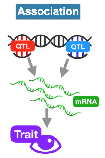
Transcriptome-wide association methods

predict expression

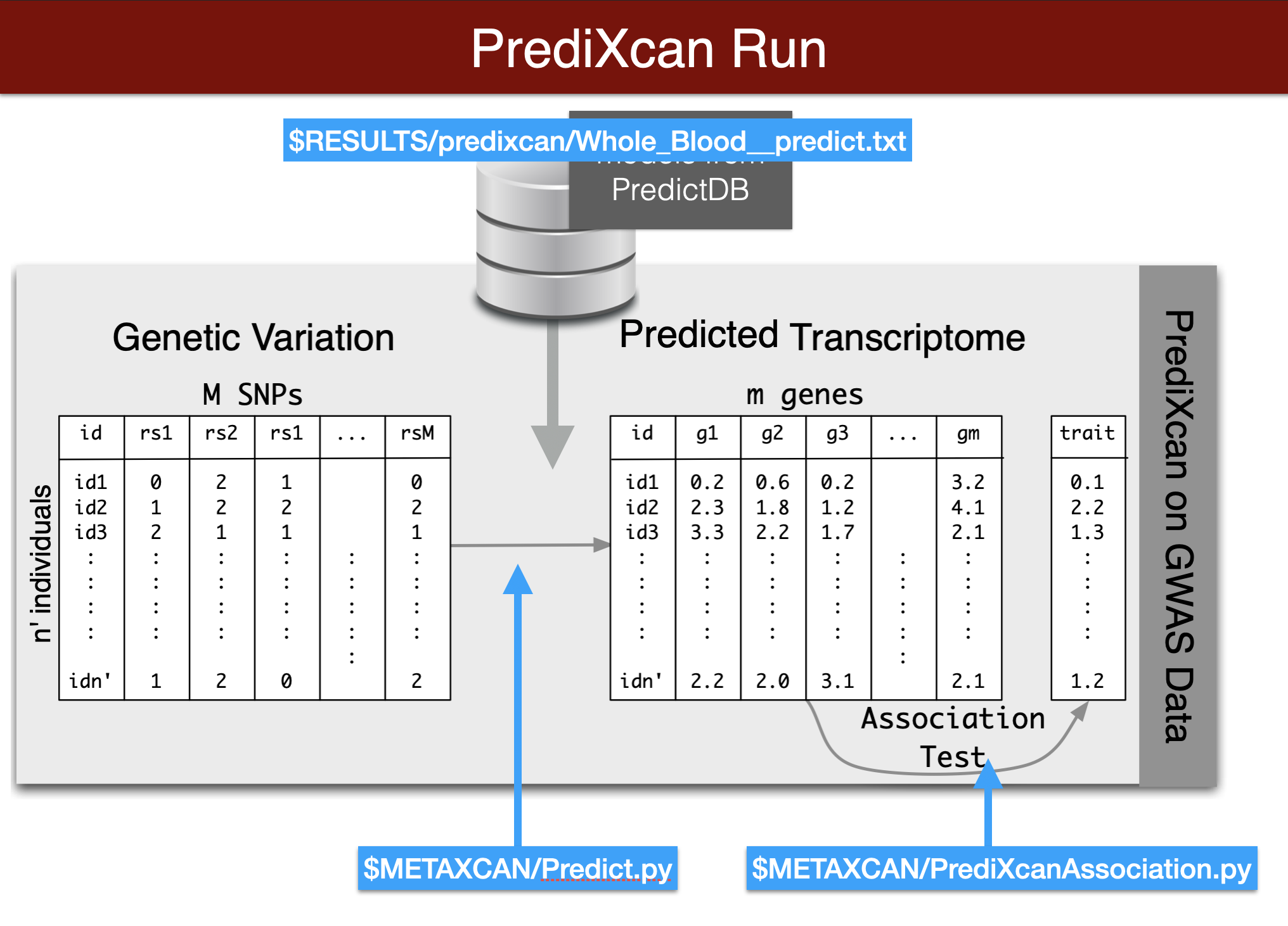
Visual summary of predixcan runs

We will predict expression of genes in whole blood using the Predict.py code in the METAXCAN folder.
Prediction models are located in the MODEL folder. Additional models for different tissues and transcriptome studies can be downloaded from predictdb.org
Remember you need to copy and paste this code chunk into the terminal to run it. Also make sure you activated the imlabtools environment which has all the necessary python modules.
Make sure all the paths and file names are correct
This run should take about one minute.
copy and paste the following block to the terminal and hit enter


printf "Predict expression\n\n"
python3 $METAXCAN/Predict.py \
--model_db_path $PRE/models/gtex_v8_en/en_Whole_Blood.db \
--vcf_genotypes $DATA/predixcan/genotype/filtered.vcf.gz \
--vcf_mode genotyped \
--variant_mapping $DATA/predixcan/gtex_v8_eur_filtered_maf0.01_monoallelic_variants.txt.gz id rsid \
--on_the_fly_mapping METADATA "chr{}_{}_{}_{}_b38" \
--prediction_output $RESULTS/predixcan/Whole_Blood__predict.txt \
--prediction_summary_output $RESULTS/predixcan/Whole_Blood__summary.txt \
--verbosity 9 \
--throw

check predicted values (run the following chunk using the green arrow)

prediction_fp = glue::glue("{RESULTS}/predixcan/Whole_Blood__predict.txt")

## Read the Predict.py output into a dataframe. This function reorganizes the data and adds gene names.
predicted_expression = load_predicted_expression(prediction_fp, gencode_df)

head(predicted_expression)

## read summary of prediction, number of SNPs per gene, cross validated prediction performance
prediction_summary = load_prediction_summary(glue::glue("{RESULTS}/predixcan/Whole_Blood__summary.txt"), gencode_df)
## number of genes with a prediction model
dim(prediction_summary)
head(prediction_summary)

print("distribution of prediction performance r2")
summary(prediction_summary$pred_perf_r2)

assess prediction performance (optional)

## download and read observed expression data from GEUVADIS 
## from https://uchicago.box.com/s/4y7xle5l0pnq9d1fwmthe2ewhogrnlrv

## Remove the version number from the gene_id's (ENSG000XXX.ver)
head(predicted_expression)

## merge predicted expression with observed expression data (by IID and gene)

## plot observes vs predicted expressioni for 
## ERAP1 (ENSG00000164307)
## PEX6 (ENSG00000124587)

## calculate spearman correlation for all genes

## what's the best performing gene?

run association with a simulated phenotype

$Y = \sum_k T_k \beta_k + \epsilon$

with random effects $\beta_k \sim (1-\pi)\cdot \delta_0 + \pi\cdot N(0,1)$


export PHENO="sim.spike_n_slab_0.01_pve0.1"

printf "association\n\n"
python3 $METAXCAN/PrediXcanAssociation.py \
--expression_file $RESULTS/predixcan/Whole_Blood__predict.txt \
--input_phenos_file $DATA/predixcan/phenotype/$PHENO.txt \
--input_phenos_column pheno \
--output $RESULTS/predixcan/$PHENO/Whole_Blood__association.txt \
--verbosity 9 \
--throw

More predicted phenotypes can be found in $DATA/predixcan/phenotype/. The naming of the phenotypes provides information about the genic architecture: the number after pve is the proportion of variance of Y explained by the genetic component of expression. The number after spike_n_slab represents the probability that a gene is causal $\pi$(i.e. prob $\beta \ne 0$)

read association results

## read association results
PHENO="sim.spike_n_slab_0.01_pve0.1"

predixcan_association = load_predixcan_association(glue::glue("{RESULTS}/predixcan/{PHENO}/Whole_Blood__association.txt"),
                                                   gencode_df)

## take a look at the results
dim(predixcan_association)
predixcan_association %>% arrange(pvalue) %>% head
predixcan_association %>% arrange(pvalue) %>% ggplot(aes(pvalue)) + geom_histogram(bins=20)
## compare distribution against the null (uniform)
gg_qqplot(predixcan_association$pvalue, max_yval = 40)

compare estimated effects with true effect sizes

truebetas = load_truebetas(glue::glue("{DATA}/predixcan/phenotype/gene-effects/{PHENO}.txt"), gencode_df)
betas = (predixcan_association %>% 
               inner_join(truebetas,by=c("gene"="gene_id")) %>%
               select(c('estimated_beta'='effect', 
                        'true_beta'='effect_size',
                        'pvalue', 
                        'gene_id'='gene', 
                        'gene_name'='gene_name.x', 
                        'region_id'='region_id.x')))
betas %>% arrange(pvalue) %>% head
## do you see examples of potential LD contamination?
betas %>% ggplot(aes(estimated_beta, true_beta))+geom_point()+geom_abline()

Summary PrediXcan

Now we will use the summary results from a GWAS of coronary artery disease to calculate the association between the genetic component of the expression of genes and coronary artery disease risk. We will use the SPrediXcan.py.

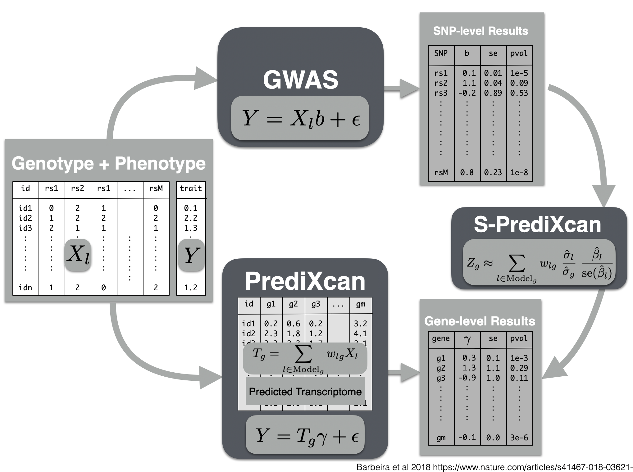
Visual summary of s-predixcan

harmonized and imputed GWAS result for coronary artery disease is available in $PRE/spredixcan/data/

run s-predixcan

python $METAXCAN/SPrediXcan.py \
--gwas_file  $DATA/spredixcan/imputed_CARDIoGRAM_C4D_CAD_ADDITIVE.txt.gz \
--snp_column panel_variant_id --effect_allele_column effect_allele --non_effect_allele_column non_effect_allele --zscore_column zscore \
--model_db_path $MODEL/gtex_v8_mashr/mashr_Whole_Blood.db \
--covariance $MODEL/gtex_v8_mashr/mashr_Whole_Blood.txt.gz \
--keep_non_rsid --additional_output --model_db_snp_key varID \
--throw \
--output_file $RESULTS/spredixcan/eqtl/CARDIoGRAM_C4D_CAD_ADDITIVE__PM__Whole_Blood.csv

plot and interpret s-predixcan results

spredixcan_association = load_spredixcan_association(glue::glue("{RESULTS}/spredixcan/eqtl/CARDIoGRAM_C4D_CAD_ADDITIVE__PM__Whole_Blood.csv"), gencode_df)
dim(spredixcan_association)
spredixcan_association %>% arrange(pvalue) %>% head
spredixcan_association %>% arrange(pvalue) %>% ggplot(aes(pvalue)) + geom_histogram(bins=20)

gg_qqplot(spredixcan_association$pvalue)

SORT1, considered to be a causal gene for LDL cholesterol and as a consequence of coronary artery disease, is not found here. Why? (tissue)

Exercise

run s-predixcan with liver model, do you find SORT1? Is it significant?
compare zscores in liver and whole blood.

run multixcan (optional)

multixcan aggregates information across multiple tissues to boost the power to detect association. It was developed movivated by the fact that eQTLs are shared across multiple tissues, i.e. many genetic variants that regulate expression are common across tissues.

python $METAXCAN/SMulTiXcan.py \
--models_folder $MODEL/gtex_v8_mashr \
--models_name_pattern "mashr_(.*).db" \
--snp_covariance $MODEL/gtex_v8_expression_mashr_snp_smultixcan_covariance.txt.gz \
--metaxcan_folder $RESULTS/spredixcan/eqtl/ \
--metaxcan_filter "CARDIoGRAM_C4D_CAD_ADDITIVE__PM__(.*).csv" \
--metaxcan_file_name_parse_pattern "(.*)__PM__(.*).csv" \
--gwas_file $DATA/spredixcan/imputed_CARDIoGRAM_C4D_CAD_ADDITIVE.txt.gz \
--snp_column panel_variant_id --effect_allele_column effect_allele --non_effect_allele_column non_effect_allele --zscore_column zscore --keep_non_rsid --model_db_snp_key varID \
--cutoff_condition_number 30 \
--verbosity 7 \
--throw \
--output $RESULTS/smultixcan/eqtl/CARDIoGRAM_C4D_CAD_ADDITIVE_smultixcan.txt

Colocalization methods

Colocalization methods seek to estimate the probability that the complex trait and expression causal variants are the same. We favor methods that calculate the probability of causality for each trait (posterior inclusion probability), called fine-mapping methods. Here we use torus for fine-mapping and fastENLOC for colocalization.

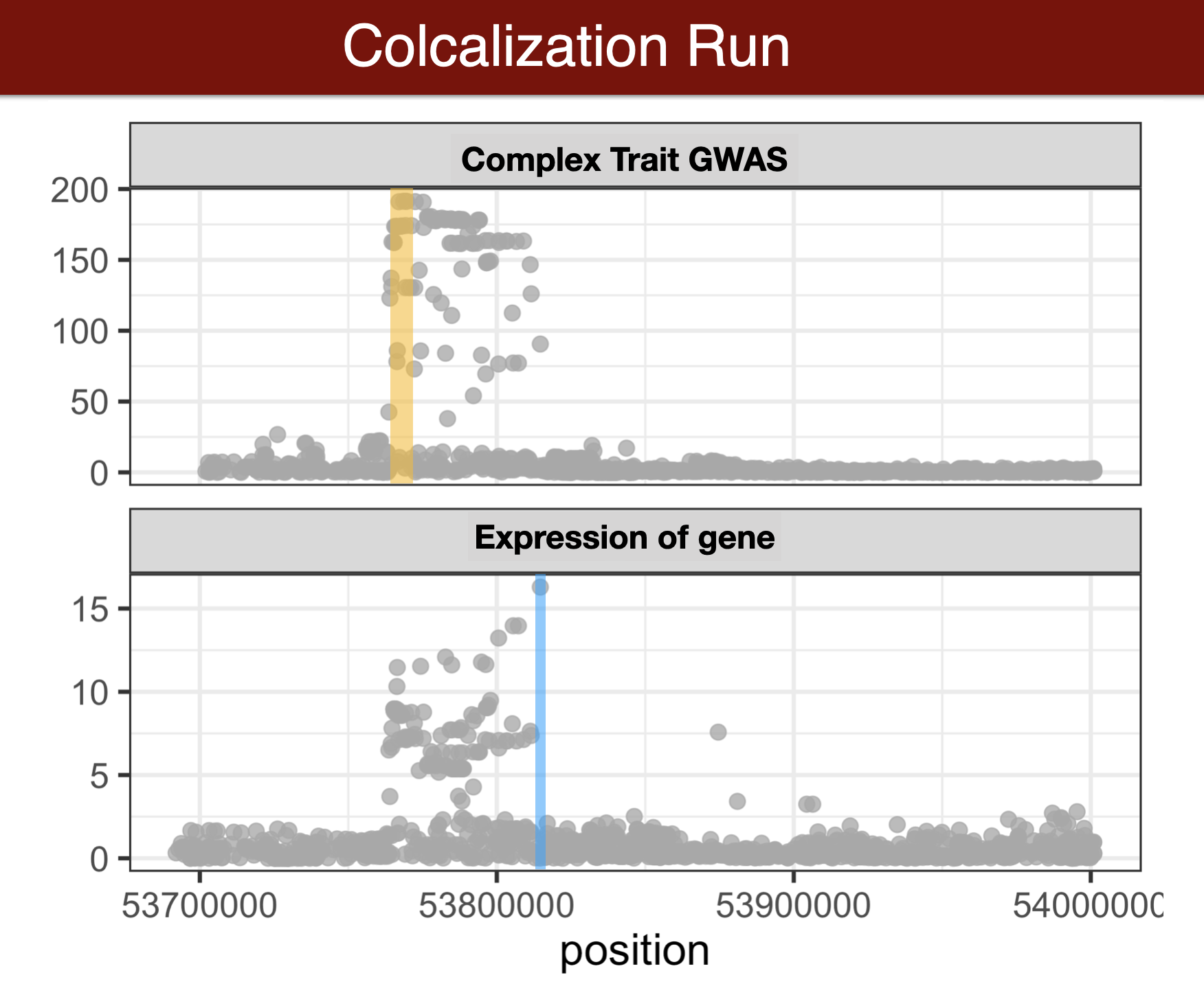
Visual summary of colocalization

GWAS summary statistics to torus format

the following code will format GWAS summary statistics into a format that the fine-mapping method torus can understand.
we precalculated this for you so there is no need to recalculate

## We ran this formatting for you because it takes over 10 minutes.
python $CODE/gwas_to_torus_zscore.py \
-input_gwas $DATA/spredixcan/imputed_CARDIoGRAM_C4D_CAD_ADDITIVE.txt.gz \
-input_ld_regions $DATA/spredixcan/eur_ld_hg38.txt.gz \
-output_fp $DATA/fastenloc/CARDIoGRAM_C4D_CAD_ADDITIVE.zval.gz

fine-map GWAS results

We will run torus due to time limitation but ideally we would like to run a method that allows multiple causal variants per locus, such as DAP-G or SusieR.
torus has been precompiled and placed within the PATH

export TORUSOFT=torus

$TORUSOFT -d $PRE/data/fastenloc/CARDIoGRAM_C4D_CAD_ADDITIVE.zval.gz --load_zval -dump_pip $PRE/data/fastenloc/CARDIoGRAM_C4D_CAD_ADDITIVE.gwas.pip
cd $PRE/data/fastenloc
gzip CARDIoGRAM_C4D_CAD_ADDITIVE.gwas.pip
cd $PRE

We can take a quick look at the z-values and finemapping PIPs:

cd $PRE/data/fastenloc
zless CARDIoGRAM_C4D_CAD_ADDITIVE.zval.gz
zless CARDIoGRAM_C4D_CAD_ADDITIVE.gwas.pip.gz

calculate colocalization with fastENLOC

## check out tutorial https://github.com/xqwen/fastenloc/tree/master/tutorial

export eqtl_annotation_gzipped=$PRE/data/fastenloc/FASTENLOC-gtex_v8.eqtl_annot.vcf.gz
export gwas_data_gzipped=$PRE/data/fastenloc/CARDIoGRAM_C4D_CAD_ADDITIVE.gwas.pip.gz
export TISSUE=Whole_Blood
export FASTENLOCSOFT=fastenloc
##export FASTENLOCSOFT=/Users/owenmelia/projects/finemapping_bin/src/fastenloc/src/fastenloc

mkdir $RESULTS/fastenloc/
cd $RESULTS/fastenloc/
$FASTENLOCSOFT -eqtl $eqtl_annotation_gzipped -gwas $gwas_data_gzipped -t $TISSUE 

#[-total_variants total_snp] [-thread n] [-prefix prefix_name] [-s shrinkage]

analyze results

## optional - compare with s-predixcan results

fastenloc_results = load_fastenloc_coloc_result(glue::glue("{RESULTS}/fastenloc/enloc.sig.out"))
spredixcan_and_fastenloc = inner_join(spredixcan_association, fastenloc_results, by=c('gene'='Signal'))
ggplot(spredixcan_and_fastenloc, aes(RCP, -log10(pvalue))) + geom_point()

## which genes are both colocalized (rcp>0.10) and significantly associated (pvalue<0.05/number of tests)

Mendelian randomization methods

run TWMR (for a locus)

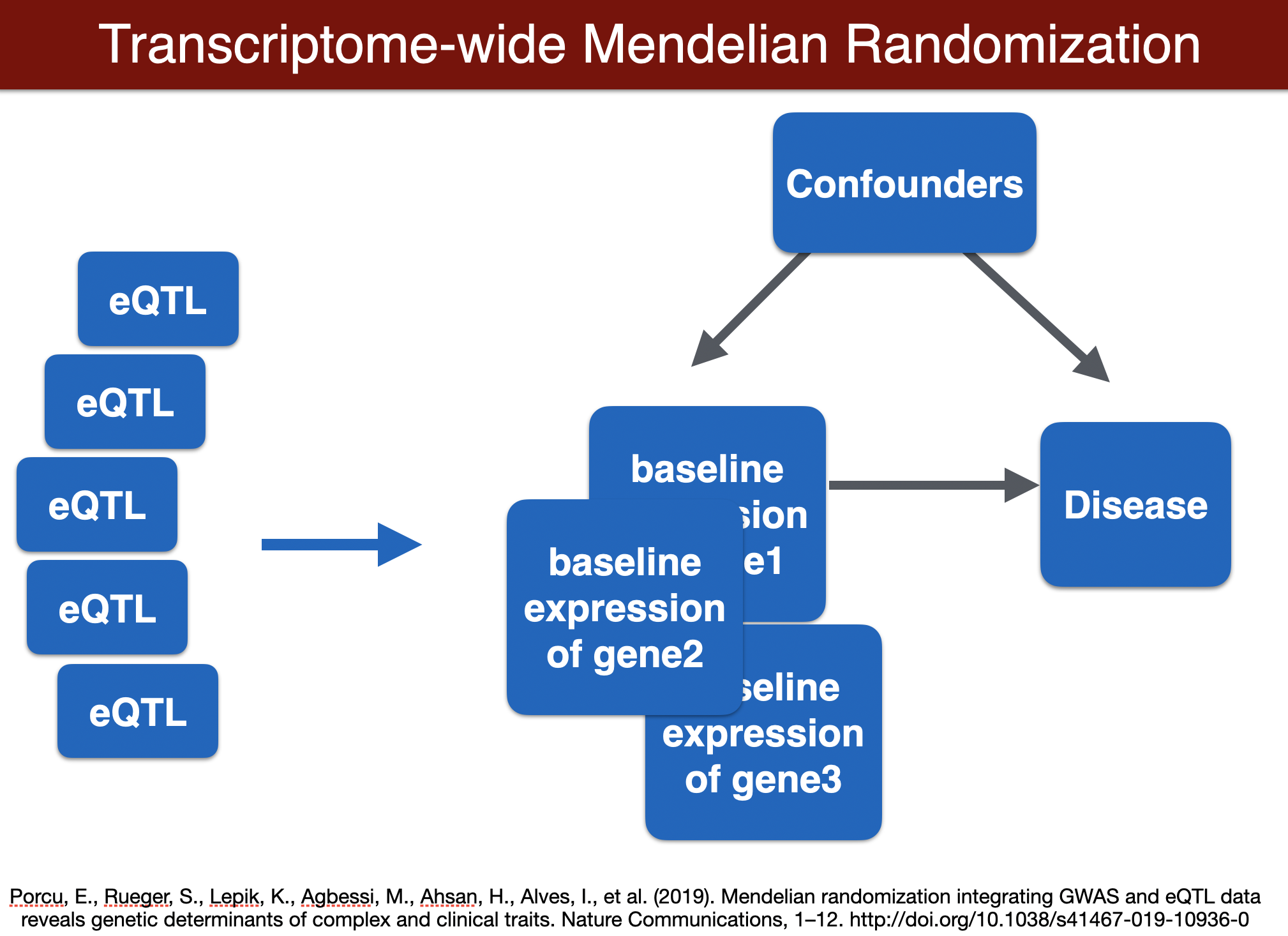
TWMR

# Load the 'analyseMR' function
source(glue::glue("{CODE}/TWMR_script.R"))

# Collect the list of genes available to run
gene_lst <- list.files(TWMR)
gene_lst <- gene_lst[str_detect(gene_lst, "ENS.*")]
gene_lst <- (gsub("\\..*", "", gene_lst) %>% unique)

# Set the gene and run. The function writes output to a file.
for (gene in gene_lst) {
  analyseMR(gene, TWMR)
}

twmr_results <- load_twmr_results(TWMR, gencode_df)

sessionInfo()

R version 3.6.0 (2019-04-26)
Platform: x86_64-apple-darwin15.6.0 (64-bit)
Running under: macOS Mojave 10.14.6

Matrix products: default
BLAS:   /Library/Frameworks/R.framework/Versions/3.6/Resources/lib/libRblas.0.dylib
LAPACK: /Library/Frameworks/R.framework/Versions/3.6/Resources/lib/libRlapack.dylib

locale:
[1] en_US.UTF-8/en_US.UTF-8/en_US.UTF-8/C/en_US.UTF-8/en_US.UTF-8

attached base packages:
[1] stats     graphics  grDevices utils     datasets  methods   base     

loaded via a namespace (and not attached):
 [1] Rcpp_1.0.5      rstudioapi_0.11 whisker_0.4     knitr_1.29     
 [5] magrittr_1.5    workflowr_1.6.2 R6_2.4.1        rlang_0.4.7    
 [9] stringr_1.4.0   tools_3.6.0     xfun_0.15       git2r_0.27.1   
[13] htmltools_0.5.0 ellipsis_0.3.1  yaml_2.2.1      digest_0.6.25  
[17] rprojroot_1.3-2 tibble_3.0.3    lifecycle_0.2.0 crayon_1.3.4   
[21] later_1.1.0.1   vctrs_0.3.1     promises_1.1.1  fs_1.4.2       
[25] glue_1.4.1      evaluate_0.14   rmarkdown_2.3   stringi_1.4.6  
[29] compiler_3.6.0  pillar_1.4.6    backports_1.1.8 httpuv_1.5.4   
[33] pkgconfig_2.0.3

QGT-Columbia-analysis-plan

Hae Kyung Im

2020-06-10