L3-Multiple-Testing

Last updated: 2020-01-15

Checks: 6 0

Knit directory: hgen471/

This reproducible R Markdown analysis was created with workflowr (version 1.3.0). The Checks tab describes the reproducibility checks that were applied when the results were created. The Past versions tab lists the development history.

R Markdown file: up-to-date

Great! Since the R Markdown file has been committed to the Git repository, you know the exact version of the code that produced these results.

Environment: empty

Great job! The global environment was empty. Objects defined in the global environment can affect the analysis in your R Markdown file in unknown ways. For reproduciblity it’s best to always run the code in an empty environment.

Seed: set.seed(20200105)

The command set.seed(20200105) was run prior to running the code in the R Markdown file. Setting a seed ensures that any results that rely on randomness, e.g. subsampling or permutations, are reproducible.

Session information: recorded

Great job! Recording the operating system, R version, and package versions is critical for reproducibility.

Cache: none

Nice! There were no cached chunks for this analysis, so you can be confident that you successfully produced the results during this run.

Repository version: bee3a31

Great! You are using Git for version control. Tracking code development and connecting the code version to the results is critical for reproducibility. The version displayed above was the version of the Git repository at the time these results were generated.

Note that you need to be careful to ensure that all relevant files for the analysis have been committed to Git prior to generating the results (you can use wflow_publish or wflow_git_commit). workflowr only checks the R Markdown file, but you know if there are other scripts or data files that it depends on. Below is the status of the Git repository when the results were generated:


Ignored files:
    Ignored:    .DS_Store
    Ignored:    .Rhistory
    Ignored:    .Rproj.user/
    Ignored:    docs/.DS_Store

Note that any generated files, e.g. HTML, png, CSS, etc., are not included in this status report because it is ok for generated content to have uncommitted changes.

These are the previous versions of the R Markdown and HTML files. If you’ve configured a remote Git repository (see ?wflow_git_remote), click on the hyperlinks in the table below to view them.

File	Version	Author	Date	Message
html	63bbad7	Hae Kyung Im	2020-01-15	Build site.
Rmd	ed556cf	Hae Kyung Im	2020-01-15	wflow_publish(all = TRUE)
html	ed556cf	Hae Kyung Im	2020-01-15	wflow_publish(all = TRUE)
Rmd	e4490eb	hakyimlab	2020-01-14	winners
html	e4490eb	hakyimlab	2020-01-14	winners
Rmd	b5bd1ad	hakyimlab	2020-01-14	winners
html	b5bd1ad	hakyimlab	2020-01-14	winners
html	0734fad	hakyimlab	2020-01-14	null p winners curse
Rmd	0c53a5b	hakyimlab	2020-01-14	null p winners curse
html	0c53a5b	hakyimlab	2020-01-14	null p winners curse

library(tidyverse)

Registered S3 methods overwritten by 'ggplot2':
  method         from 
  [.quosures     rlang
  c.quosures     rlang
  print.quosures rlang

── Attaching packages ────────────────────────────── tidyverse 1.2.1 ──

✔ ggplot2 3.1.1     ✔ purrr   0.3.2
✔ tibble  2.1.2     ✔ dplyr   0.8.1
✔ tidyr   0.8.3     ✔ stringr 1.4.0
✔ readr   1.3.1     ✔ forcats 0.4.0

── Conflicts ───────────────────────────────── tidyverse_conflicts() ──
✖ dplyr::filter() masks stats::filter()
✖ dplyr::lag()    masks stats::lag()

fastlm = function(xx,yy)
{
  ## compute betahat (regression coef) and pvalue with Ftest
  ## for now it does not take covariates

  df1 = 2
  df0 = 1
  ind = !is.na(xx) & !is.na(yy)
  xx = xx[ind]
  yy = yy[ind]
  n = sum(ind)
  xbar = mean(xx)
  ybar = mean(yy)
  xx = xx - xbar
  yy = yy - ybar

  SXX = sum( xx^2 )
  SYY = sum( yy^2 )
  SXY = sum( xx * yy )

  betahat = SXY / SXX

  RSS1 = sum( ( yy - xx * betahat )^2 )
  RSS0 = SYY

  fstat = ( ( RSS0 - RSS1 ) / ( df1 - df0 ) )  / ( RSS1 / ( n - df1 ) )
  pval = 1 - pf(fstat, df1 = ( df1 - df0 ), df2 = ( n - df1 ))
  res = list(betahat = betahat, pval = pval)

  return(res)
}

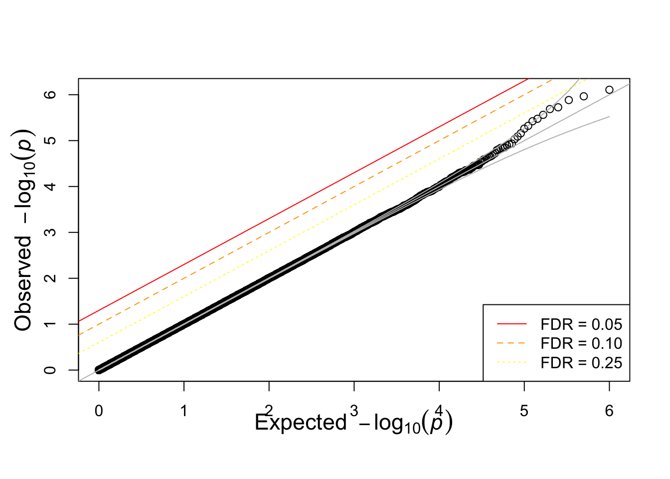
## pvalue vs uniform

qqunif = 
function(p,BH=T,CI=T,...)
{
  p=na.omit(p)
  nn = length(p)
  xx =  -log10((1:nn)/(nn+1))
  plot( xx,  -sort(log10(p)),
     xlab=expression(Expected~~-log[10](italic(p))),
        ylab=expression(Observed~~-log[10](italic(p))),
       cex.lab=1.4,mgp=c(2,1,0),
       ... )
  abline(0,1,col='gray')
  if(BH)
    {
      abline(-log10(0.05),1, col='red',lty=1)
      abline(-log10(0.10),1, col='orange',lty=2)
      abline(-log10(0.25),1, col='yellow',lty=3)
      legend('bottomright', c("FDR = 0.05","FDR = 0.10","FDR = 0.25"),
             col=c('red','orange','yellow'),lty=1:3, cex=1)
      abline(h=-log10(0.05/nn)) ## bonferroni
    }
  if(CI)
  {
    ## create the confidence intervals
    c95 <- rep(0,nn)
    c05 <- rep(0,nn)
    ## the jth order statistic from a
    ## uniform(0,1) sample
    ## has a beta(j,n-j+1) distribution
    ## (Casella & Berger, 2002,
    ## 2nd edition, pg 230, Duxbury)
    ## this portion was posted by anonymous on
    ## http://gettinggeneticsdone.blogspot.com/2009/11/qq-plots-of-p-values-in-r-using-ggplot2.html
    
    for(i in 1:nn)
    {
      c95[i] <- qbeta(0.95,i,nn-i+1)
      c05[i] <- qbeta(0.05,i,nn-i+1)
    }

    lines(xx,-log10(c95),col='gray')
    lines(xx,-log10(c05),col='gray')
  }
}

calculate probability of at least one false positive (reject null when null is true)

alpha = 0.05

Patleastonemistake = function(m) {1 - (1-alpha)^m}

curve(Patleastonemistake,from = 1, to=100, ylab="Prob at least one wrong", xlab="m = number of tests")
grid()
abline(h=1,col='gray')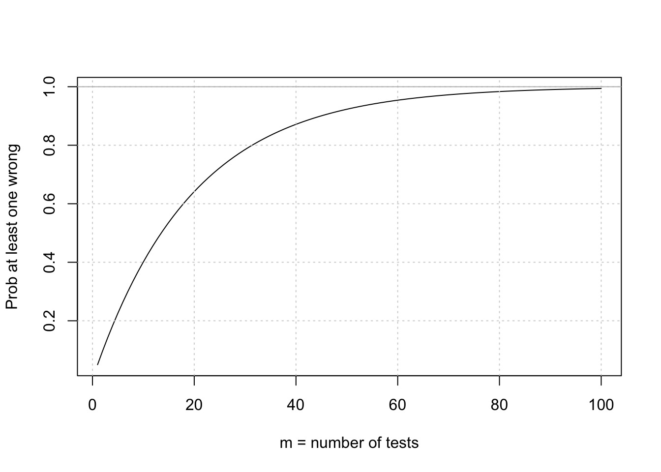

Version	Author	Date
ed556cf	Hae Kyung Im	2020-01-15
0734fad	hakyimlab	2020-01-14
0c53a5b	hakyimlab	2020-01-14

simulate a GWAS data under null (no assoc between X and Y)

nsnp = 1000000
nsam = 1000
maf = 0.30

## to simplify, we use the same maf for all SNPs in the GWAS

simGWASnull = function(nsnp,nsam,maf)
{
  Xfather = matrix( rbinom(nsam * nsnp,1,maf), nsam, nsnp )
  Xmother = matrix( rbinom(nsam * nsnp,1,maf), nsam, nsnp )
  Xboth = Xfather+ Xmother

  Y = matrix( rnorm(nsam))
  return(list(Y=Y, Xmat=Xboth))
}

simu = simGWASnull(nsnp, nsam, maf)

run GWAS by regression and show that the p-values are uniformly distributed

pvec = rep(NA,nsnp)
bvec = rep(NA,nsnp)

for(ss in 1:nsnp)
{
  fit = fastlm(simu$X[,ss], simu$Y)
  pvec[ss] = fit$pval  
  bvec[ss] = fit$betahat
}


hist(pvec,xlab="p-value",main="Histogram of p-values under Null")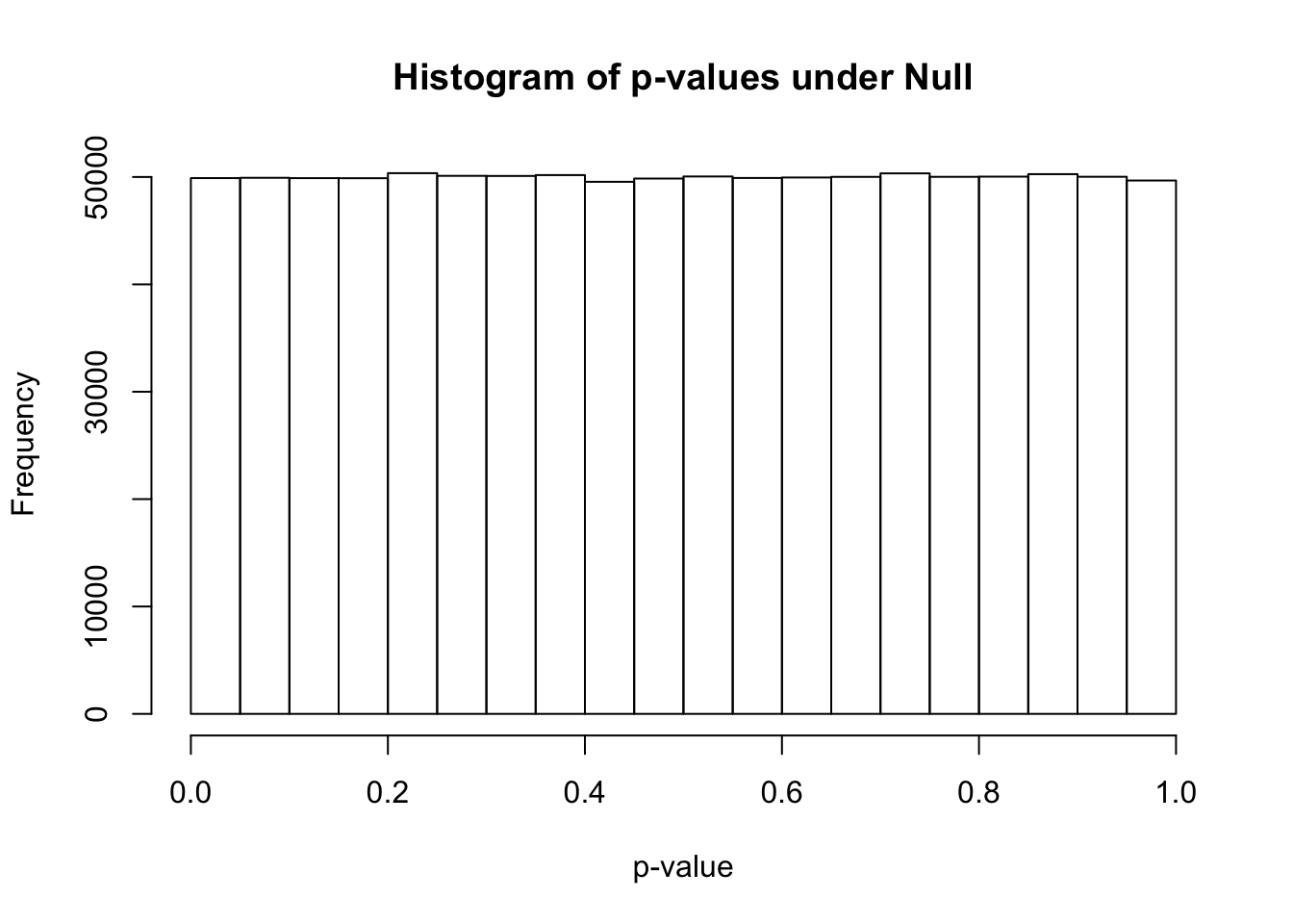

Version	Author	Date
63bbad7	Hae Kyung Im	2020-01-15

show qqplot against expected null

qqunif(pvec)

Version	Author	Date
63bbad7	Hae Kyung Im	2020-01-15

what does the most significant association look like

ind = which( pvec == min(pvec) )

boxplot(simu$Y ~ simu$X[,ind])

points(jitter(simu$X[,ind]), simu$Y, type="p")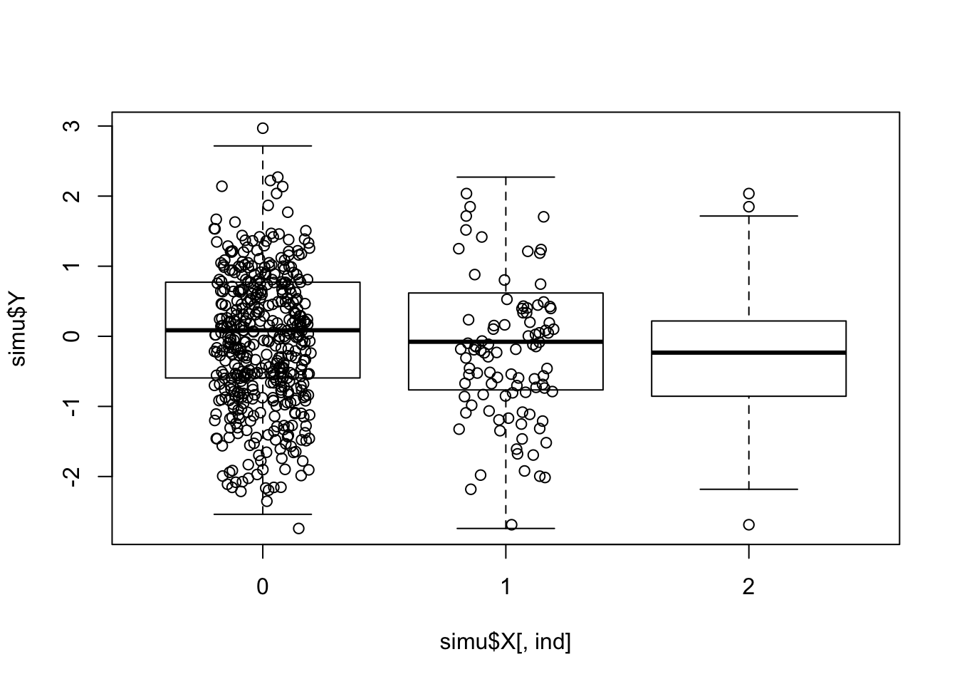

Version	Author	Date
63bbad7	Hae Kyung Im	2020-01-15

example of winner’s curse (even when effect size is 0, we get larger when we select significant SNPs)

ind = which(pvec < 0.01)

df = tibble(effect = c(bvec[ind],bvec), type = c(rep("signif",length(ind)),rep("all",length(bvec)) ) )

ggplot(df, aes(abs(effect), fill=type)) + geom_density(alpha = 0.6, color=NA) + theme_bw(base_size = 15) + ggtitle("Winner's curse")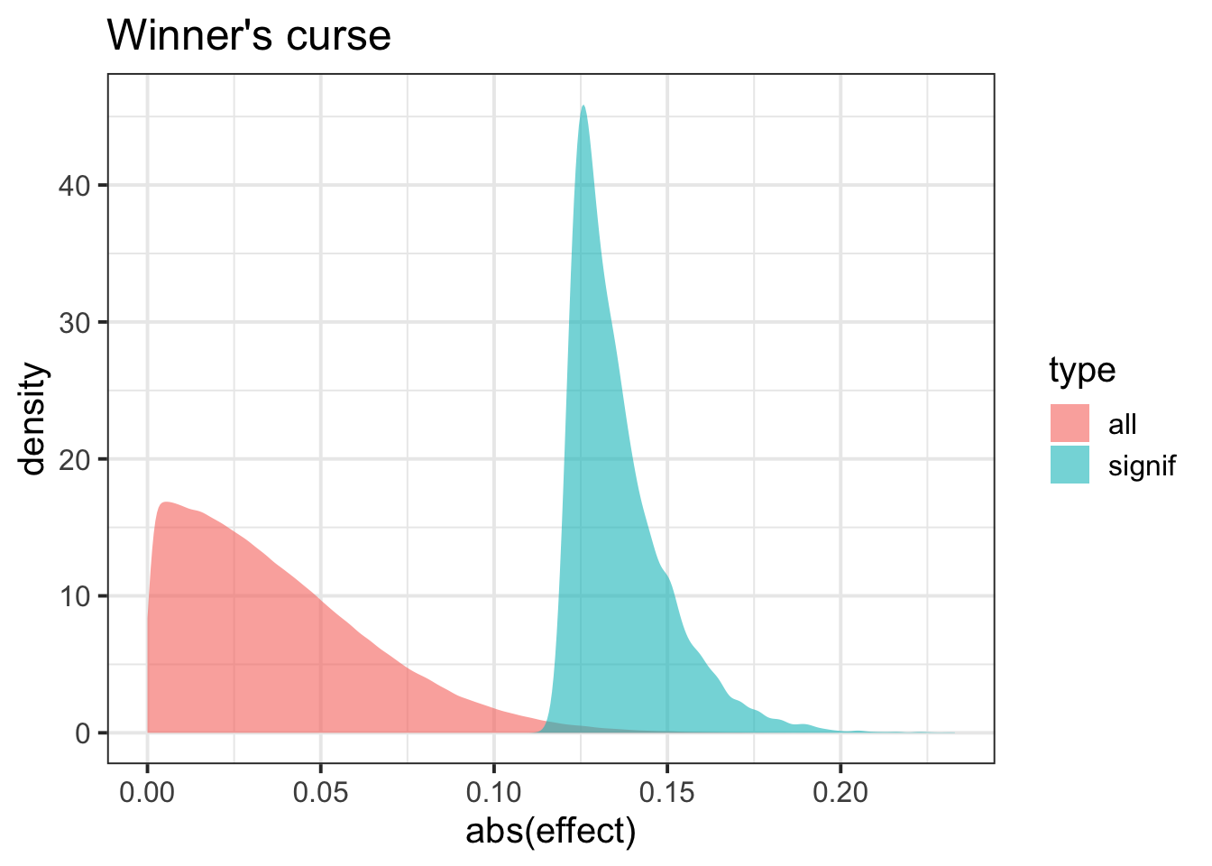

Version	Author	Date
63bbad7	Hae Kyung Im	2020-01-15

sessionInfo()

R version 3.6.0 (2019-04-26)
Platform: x86_64-apple-darwin15.6.0 (64-bit)
Running under: macOS Mojave 10.14.6

Matrix products: default
BLAS:   /Library/Frameworks/R.framework/Versions/3.6/Resources/lib/libRblas.0.dylib
LAPACK: /Library/Frameworks/R.framework/Versions/3.6/Resources/lib/libRlapack.dylib

locale:
[1] en_US.UTF-8/en_US.UTF-8/en_US.UTF-8/C/en_US.UTF-8/en_US.UTF-8

attached base packages:
[1] stats     graphics  grDevices utils     datasets  methods   base     

other attached packages:
[1] forcats_0.4.0   stringr_1.4.0   dplyr_0.8.1     purrr_0.3.2    
[5] readr_1.3.1     tidyr_0.8.3     tibble_2.1.2    ggplot2_3.1.1  
[9] tidyverse_1.2.1

loaded via a namespace (and not attached):
 [1] Rcpp_1.0.2       cellranger_1.1.0 plyr_1.8.4       pillar_1.4.1    
 [5] compiler_3.6.0   git2r_0.25.2     workflowr_1.3.0  tools_3.6.0     
 [9] digest_0.6.19    lubridate_1.7.4  jsonlite_1.6     evaluate_0.14   
[13] nlme_3.1-139     gtable_0.3.0     lattice_0.20-38  pkgconfig_2.0.2 
[17] rlang_0.4.1      cli_1.1.0        rstudioapi_0.10  yaml_2.2.0      
[21] haven_2.1.0      xfun_0.7         withr_2.1.2      xml2_1.2.0      
[25] httr_1.4.0       knitr_1.23       hms_0.4.2        generics_0.0.2  
[29] fs_1.3.1         rprojroot_1.3-2  grid_3.6.0       tidyselect_0.2.5
[33] glue_1.3.1       R6_2.4.0         readxl_1.3.1     rmarkdown_1.13  
[37] modelr_0.1.4     magrittr_1.5     whisker_0.3-2    backports_1.1.4 
[41] scales_1.0.0     htmltools_0.4.0  rvest_0.3.4      assertthat_0.2.1
[45] colorspace_1.4-1 labeling_0.3     stringi_1.4.3    lazyeval_0.2.2  
[49] munsell_0.5.0    broom_0.5.2      crayon_1.3.4