L6-population-structure

workflowr

• Summary
• Checks
• Past versions

Last updated: 2020-01-30

Checks: 6 1

Knit directory: hgen471/

This reproducible R Markdown analysis was created with workflowr (version 1.5.0). The Checks tab describes the reproducibility checks that were applied when the results were created. The Past versions tab lists the development history.

---

R Markdown file: uncommitted changes

The R Markdown file has unstaged changes. To know which version of the R Markdown file created these results, you’ll want to first commit it to the Git repo. If you’re still working on the analysis, you can ignore this warning. When you’re finished, you can run wflow_publish to commit the R Markdown file and build the HTML.

Environment: empty

Great job! The global environment was empty. Objects defined in the global environment can affect the analysis in your R Markdown file in unknown ways. For reproduciblity it’s best to always run the code in an empty environment.

Seed: set.seed(20200105)

The command set.seed(20200105) was run prior to running the code in the R Markdown file. Setting a seed ensures that any results that rely on randomness, e.g. subsampling or permutations, are reproducible.

Session information: recorded

Great job! Recording the operating system, R version, and package versions is critical for reproducibility.

Cache: none

Nice! There were no cached chunks for this analysis, so you can be confident that you successfully produced the results during this run.

File paths: relative

Great job! Using relative paths to the files within your workflowr project makes it easier to run your code on other machines.

Repository version: e73a329

Great! You are using Git for version control. Tracking code development and connecting the code version to the results is critical for reproducibility. The version displayed above was the version of the Git repository at the time these results were generated.

Note that you need to be careful to ensure that all relevant files for the analysis have been committed to Git prior to generating the results (you can use wflow_publish or wflow_git_commit). workflowr only checks the R Markdown file, but you know if there are other scripts or data files that it depends on. Below is the status of the Git repository when the results were generated:

Ignored files:
    Ignored:    .DS_Store
    Ignored:    .Rhistory
    Ignored:    .Rproj.user/
    Ignored:    analysis/.Rhistory

Unstaged changes:
    Modified:   analysis/L6-download-data.Rmd
    Modified:   analysis/L6-population-structure.Rmd

Note that any generated files, e.g. HTML, png, CSS, etc., are not included in this status report because it is ok for generated content to have uncommitted changes.

---

These are the previous versions of the R Markdown and HTML files. If you’ve configured a remote Git repository (see ?wflow_git_remote), click on the hyperlinks in the table below to view them.

File	Version	Author	Date	Message
Rmd	e73a329	Hae Kyung Im	2020-01-27	L6 examples
html	e73a329	Hae Kyung Im	2020-01-27	L6 examples

---

library(tidyverse)

── Attaching packages ─────────────────────────────── tidyverse 1.2.1 ──

✔ ggplot2 3.2.1     ✔ purrr   0.3.3
✔ tibble  2.1.3     ✔ dplyr   0.8.3
✔ tidyr   1.0.0     ✔ stringr 1.4.0
✔ readr   1.3.1     ✔ forcats 0.4.0

── Conflicts ────────────────────────────────── tidyverse_conflicts() ──
✖ dplyr::filter() masks stats::filter()
✖ dplyr::lag()    masks stats::lag()

work.dir ="~/Downloads/hapmap/"

## qqunif function
source("https://gist.githubusercontent.com/hakyim/38431b74c6c0bf90c12f/raw/21fbae9a48dc475f42fa60f0ef5509d071dea873/qqunif")

*What’s the population composition?**

popinfo = read_tsv(paste0(work.dir,"relationships_w_pops_051208.txt"))

Parsed with column specification:
cols(
  FID = col_character(),
  IID = col_character(),
  dad = col_character(),
  mom = col_character(),
  sex = col_double(),
  pheno = col_double(),
  population = col_character()
)

popinfo %>% count(population)

# A tibble: 11 x 2
   population     n
   <chr>      <int>
 1 ASW           90
 2 CEU          180
 3 CHB           90
 4 CHD          100
 5 GIH          100
 6 JPT           91
 7 LWK          100
 8 MEX           90
 9 MKK          180
10 TSI          100
11 YRI          180

samdata = read_tsv(paste0(work.dir,"phase3_corrected.psam"),guess_max = 2500) 

Parsed with column specification:
cols(
  `#IID` = col_character(),
  PAT = col_character(),
  MAT = col_character(),
  SEX = col_double(),
  SuperPop = col_character(),
  Population = col_character()
)

superpop = samdata %>% select(SuperPop,Population) %>% unique()

superpop = rbind(superpop, data.frame(SuperPop=c("EAS","HIS","AFR"),Population=c("CHD","MEX","MKK")))

Effect of population structure in Hardy Weinberg

## what happens if we calculate HWE with this mixed population?
system(glue::glue("~/bin/plink --bfile {work.dir}hapmapch22 --hardy --out {work.dir}output/allhwe"))
allhwe = read.table(glue::glue("{work.dir}output/allhwe.hwe"),header=TRUE,as.is=TRUE)
hist(allhwe$P)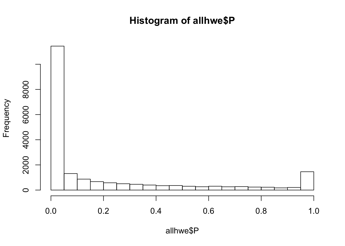

Past versions of “hardy weinberg all populations-1.png”

Version	Author	Date
e73a329	Hae Kyung Im	2020-01-27

qqunif(allhwe$P,main='HWE HapMap3 All Pop')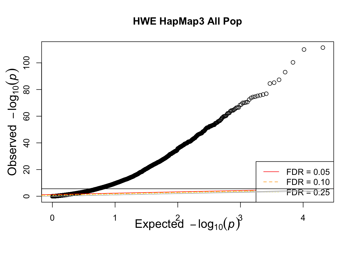

Past versions of “hardy weinberg all populations-2.png”

Version	Author	Date
e73a329	Hae Kyung Im	2020-01-27

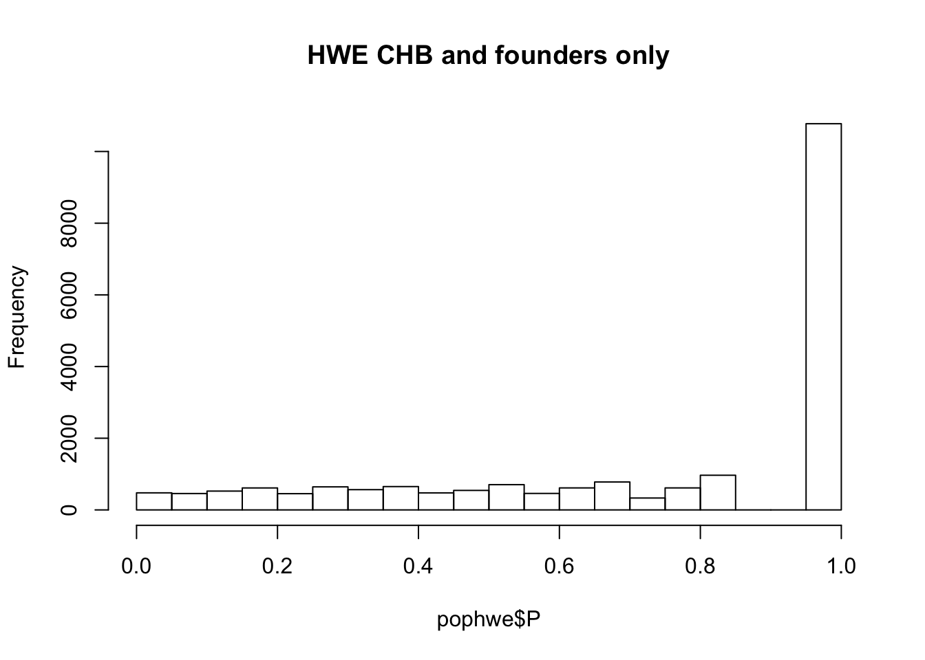
What if we calculate with single population?

pop = "CHB"
pop = "CEU"
pop = "YRI"

for(pop in c("CHB","CEU","YRI"))
{
  ## what if we calculate with single population?
  popinfo %>% filter(population==pop) %>%
    write_tsv(path=glue::glue("{work.dir}{pop}.fam") )
  system(glue::glue("~/bin/plink --bfile {work.dir}hapmapch22 --hardy --keep {work.dir}{pop}.fam --out {work.dir}output/hwe-{pop}"))
  pophwe = read.table(glue::glue("{work.dir}output/hwe-{pop}.hwe"),header=TRUE,as.is=TRUE)
  hist(pophwe$P,main=glue::glue("HWE {pop} and founders only"))
  qqunif(pophwe$P,main=glue::glue("HWE {pop} and founders only"))
}

Past versions of “hardy weinberg single population-1.png”

Version	Author	Date
e73a329	Hae Kyung Im	2020-01-27

Past versions of “hardy weinberg single population-2.png”

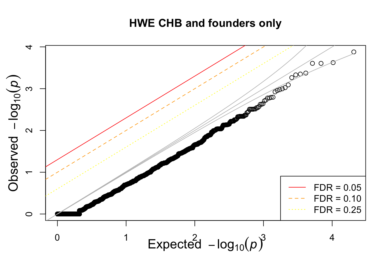
Version	Author	Date
e73a329	Hae Kyung Im	2020-01-27

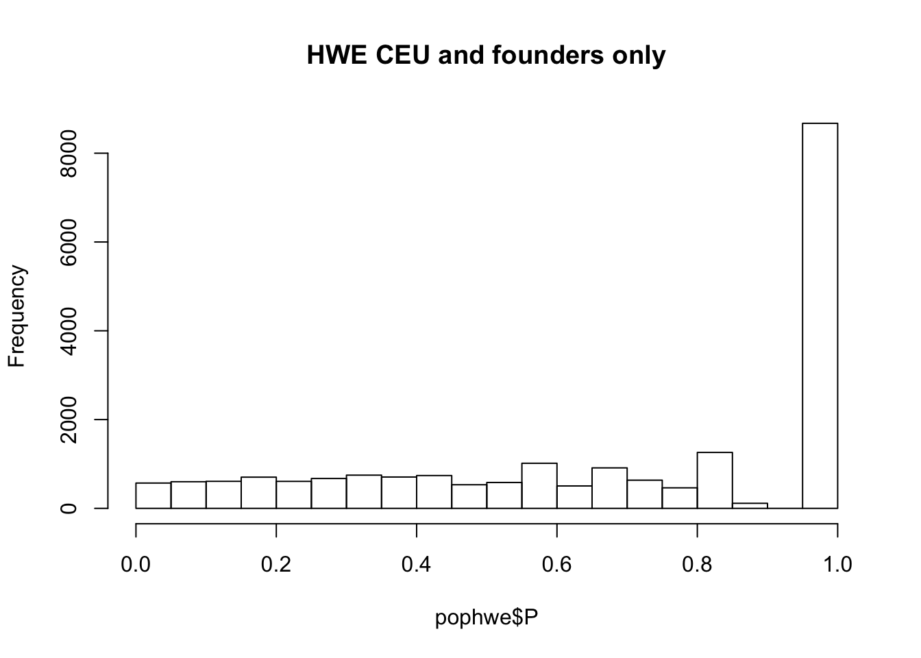
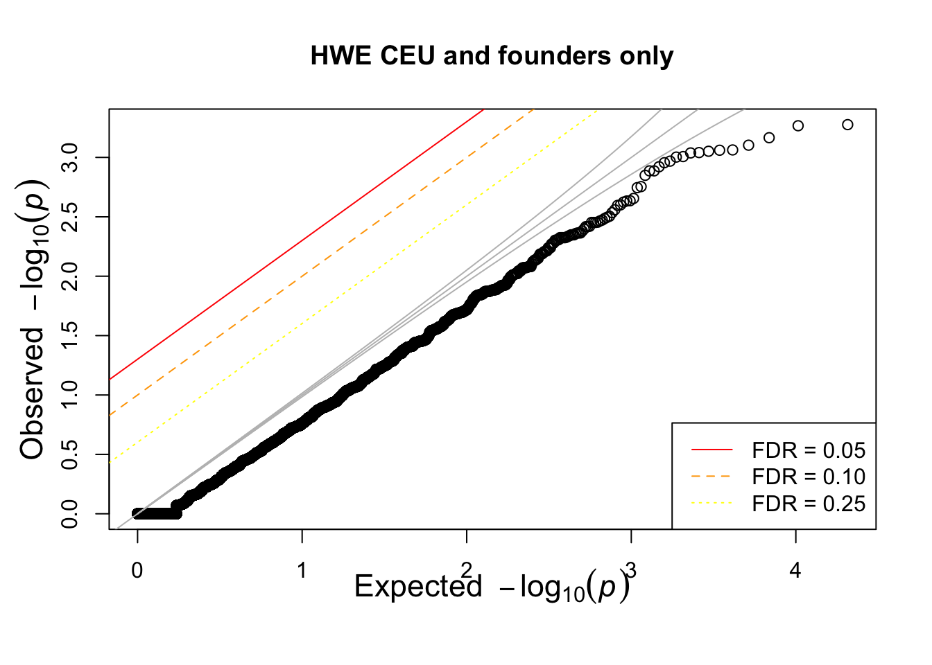
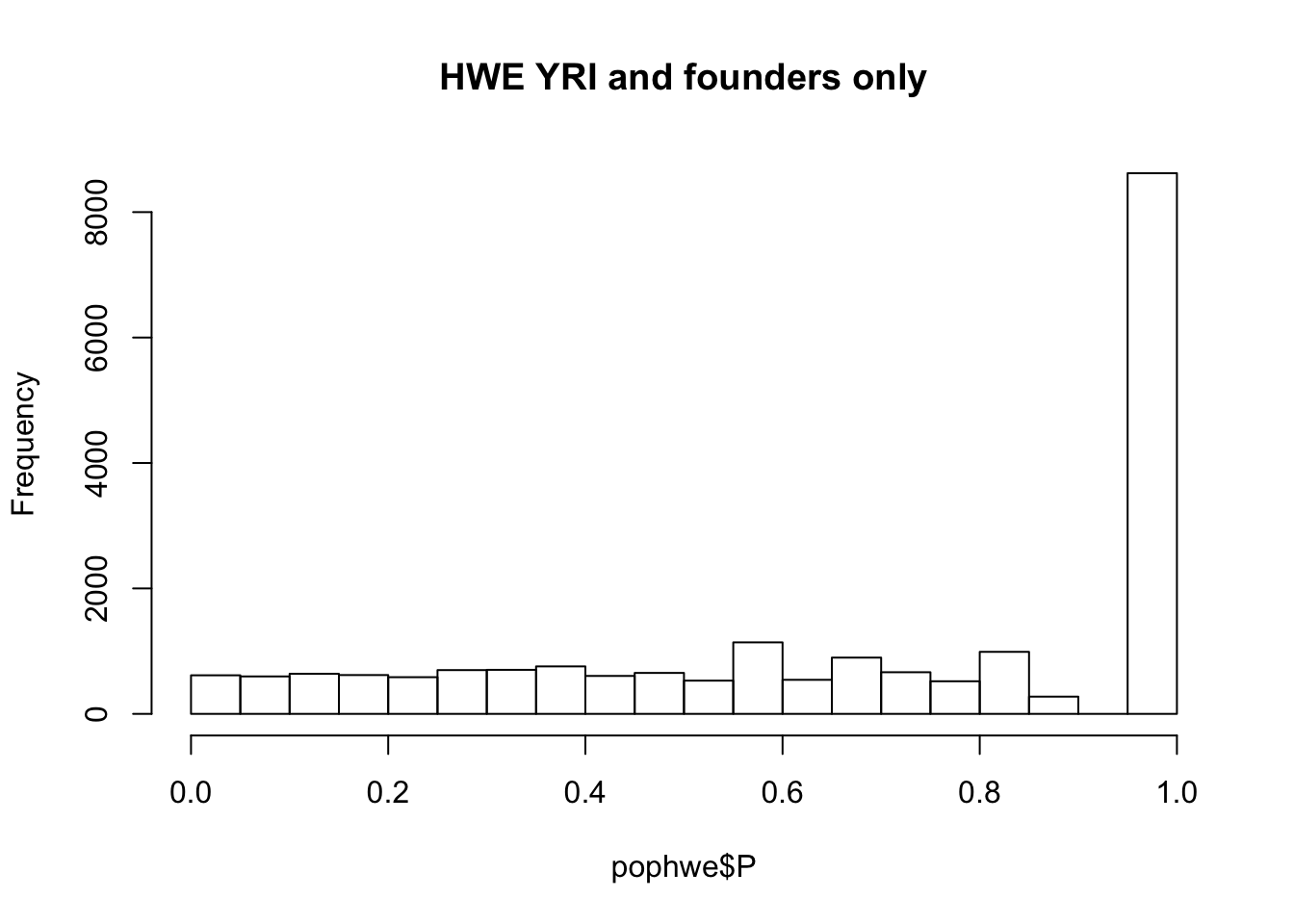
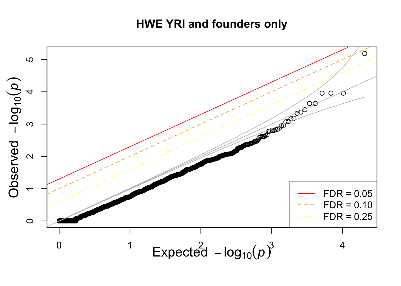
## not much difference when --nonfounders option is added

What if we add non founders? Some of the samples in HapMap were recruited from families.

## what if we add nonfounders?
system(glue::glue("~/bin/plink --bfile {work.dir}hapmapch22 --hardy --keep {work.dir}CEU.fam --nonfounders --out {work.dir}output/CEUhwe_nf"))
CEUhwe_nf = read.table(glue::glue("{work.dir}output/CEUhwe_nf.hwe"),header=TRUE,as.is=TRUE)
hist(CEUhwe_nf$P,main="HWE CEU + non founders")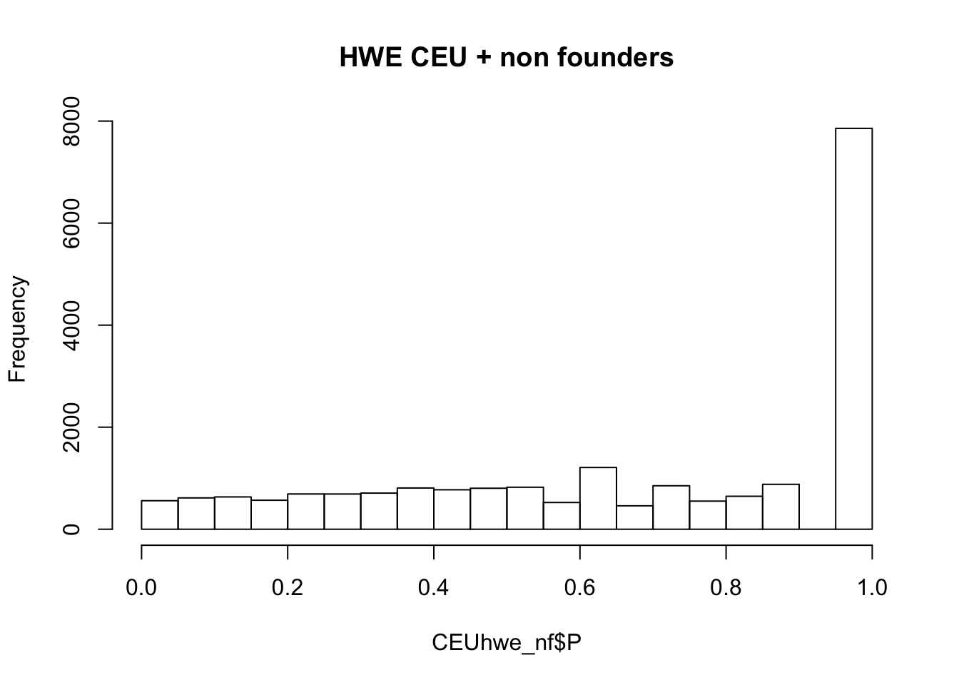

Past versions of “hardy weinberg including non founders-1.png”

Version	Author	Date
e73a329	Hae Kyung Im	2020-01-27

qqunif(CEUhwe_nf$P,main="HWE CEU + non founders")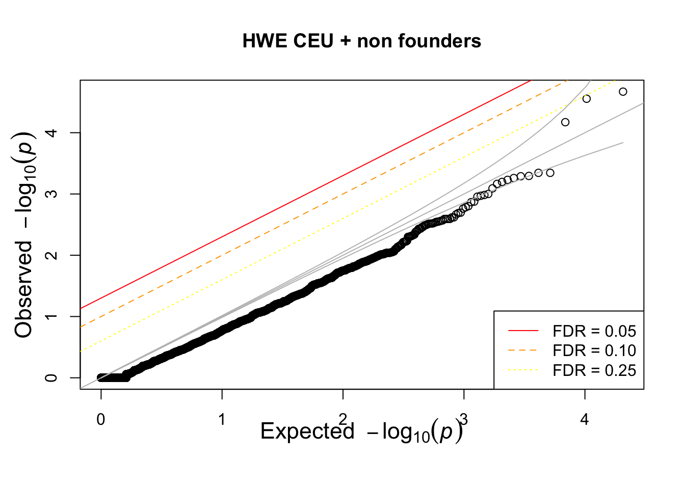

Past versions of “hardy weinberg including non founders-2.png”

Version	Author	Date
e73a329	Hae Kyung Im	2020-01-27

qqplot(-log10(CEUhwe_nf$P),-log10(CEUhwe_nf$P),main="all vs founders only" );abline(0,1)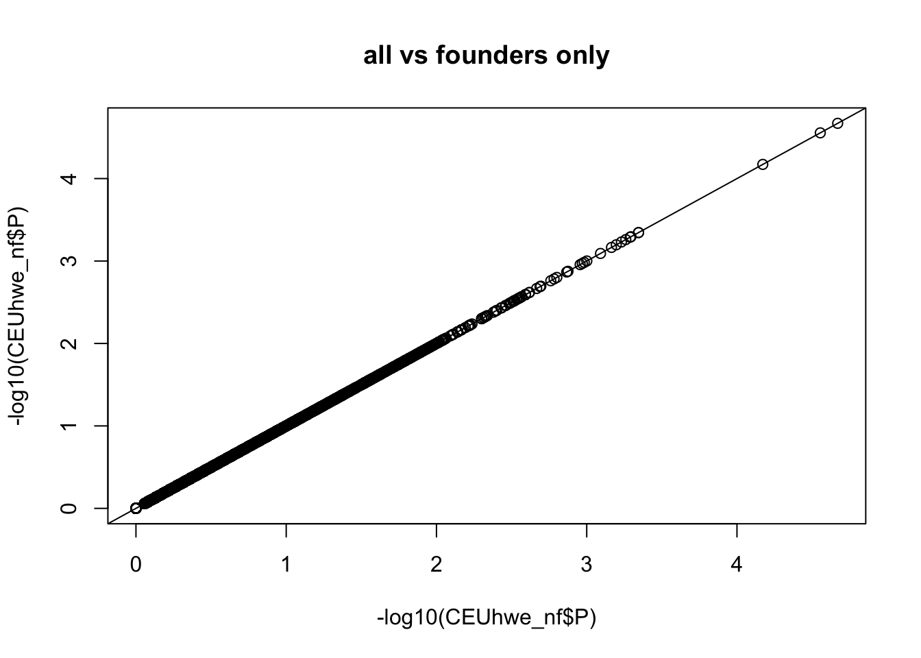 

Past versions of “hardy weinberg including non founders-3.png”

Version	Author	Date
e73a329	Hae Kyung Im	2020-01-27

GWAS on a growth phenotype in HapMap samples

## read igrowth
igrowth = read_tsv("https://raw.githubusercontent.com/hakyimlab/igrowth/master/rawgrowth.txt")

Parsed with column specification:
cols(
  IID = col_character(),
  sex = col_double(),
  pop = col_character(),
  experim = col_double(),
  meas.by = col_double(),
  serum = col_character(),
  growth = col_double()
)

## fix FID from igrowth file
igrowth = popinfo %>% select(-pheno) %>% inner_join(igrowth %>% select(IID,growth), by=c("IID"="IID"))
write_tsv(igrowth,path=glue::glue("{work.dir}igrowth.pheno"))
igrowth %>% ggplot(aes(population,growth)) + geom_violin(aes(fill=population)) + geom_boxplot(width=0.2,col='black',fill='gray',alpha=.8) + theme_bw(base_size = 15)

Warning: Removed 130 rows containing non-finite values (stat_ydensity).

Warning: Removed 130 rows containing non-finite values (stat_boxplot).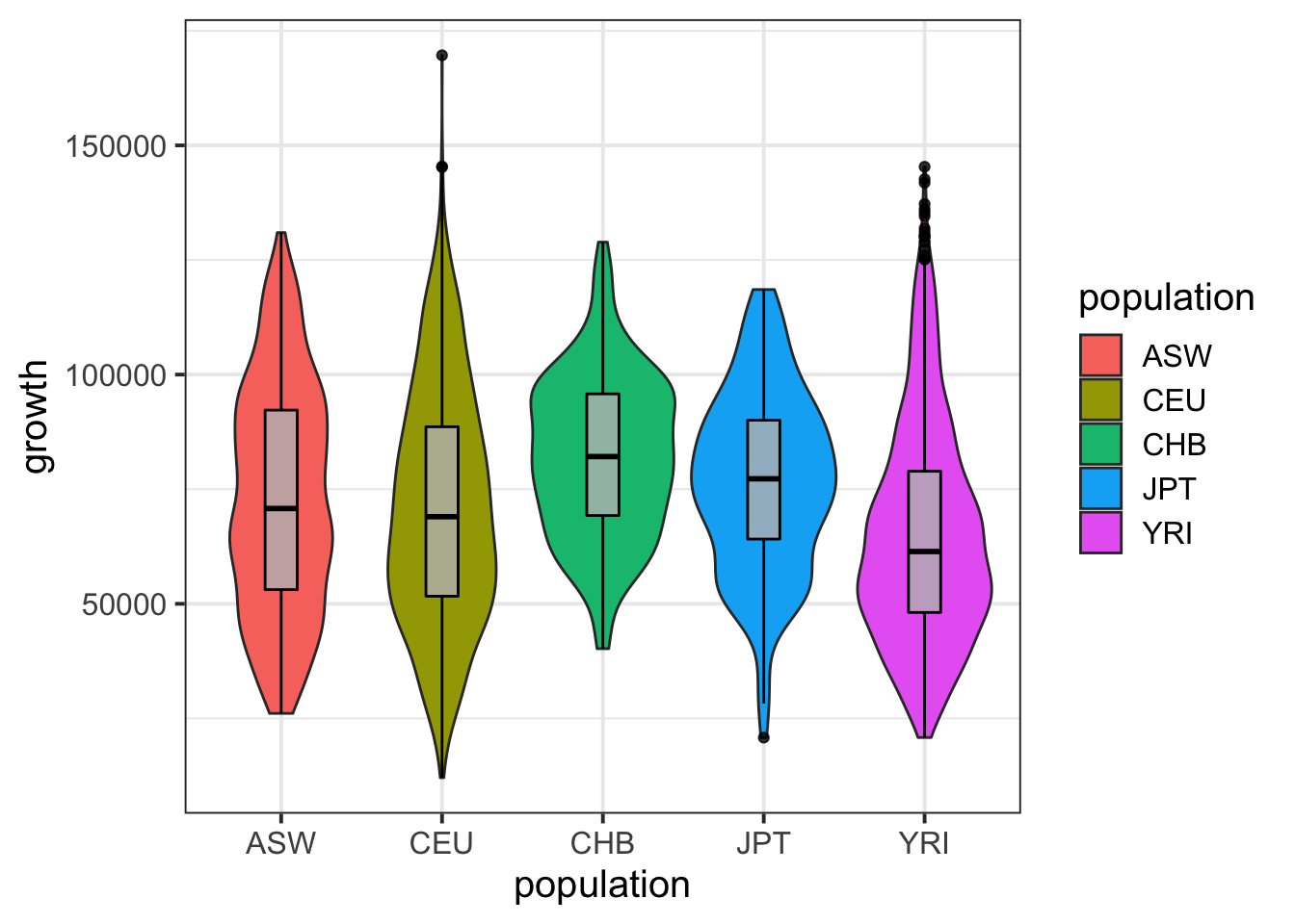

Past versions of “intrinsic growth phenotype GWAS-1.png”

Version	Author	Date
e73a329	Hae Kyung Im	2020-01-27

summary( lm(growth~population,data=igrowth) )

Call:
lm(formula = growth ~ population, data = igrowth)

Residuals:
   Min     1Q Median     3Q    Max 
-58821 -18093  -2242  15896  98760 

Coefficients:
              Estimate Std. Error t value Pr(>|t|)    
(Intercept)    73080.8      938.2  77.894  < 2e-16 ***
populationCEU  -2190.1     1175.4  -1.863   0.0625 .  
populationCHB   9053.1     2043.9   4.429 9.73e-06 ***
populationJPT   3476.8     2034.8   1.709   0.0876 .  
populationYRI  -7985.2     1137.2  -7.022 2.61e-12 ***
---
Signif. codes:  0 '***' 0.001 '**' 0.01 '*' 0.05 '.' 0.1 ' ' 1

Residual standard error: 24160 on 3591 degrees of freedom
  (130 observations deleted due to missingness)
Multiple R-squared:  0.0345,    Adjusted R-squared:  0.03342 
F-statistic: 32.08 on 4 and 3591 DF,  p-value: < 2.2e-16

system(glue::glue("~/bin/plink --bfile {work.dir}hapmapch22 --linear --pheno {work.dir}igrowth.pheno --pheno-name growth --maf 0.05 --out {work.dir}output/igrowth"))
igrowth.assoc = read.table(glue::glue("{work.dir}output/igrowth.assoc.linear"),header=T,as.is=T)
hist(igrowth.assoc$P)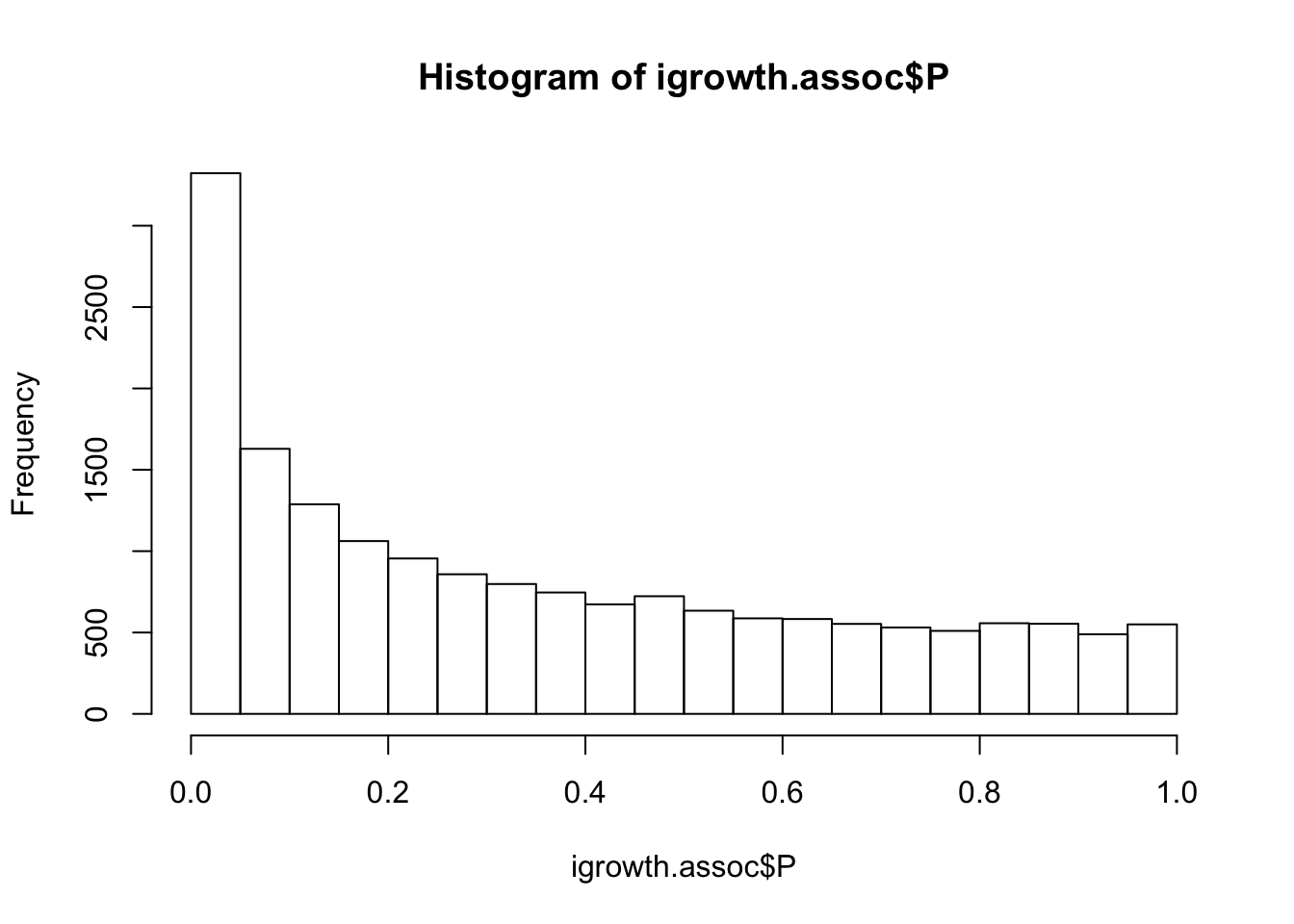

Past versions of “intrinsic growth phenotype GWAS-2.png”

Version	Author	Date
e73a329	Hae Kyung Im	2020-01-27

qqunif(igrowth.assoc$P)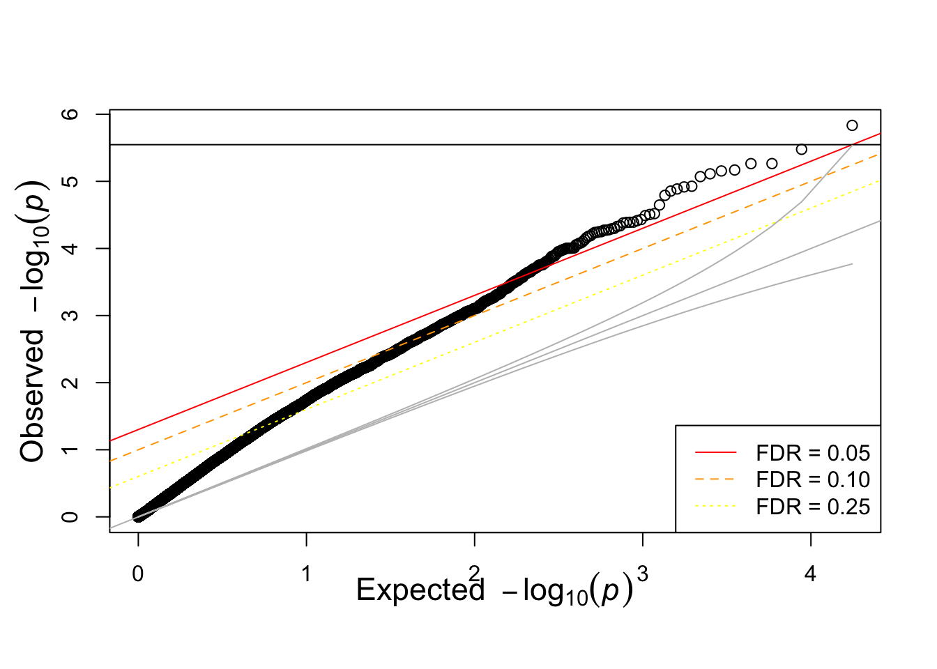

Past versions of “intrinsic growth phenotype GWAS-3.png”

Version	Author	Date
e73a329	Hae Kyung Im	2020-01-27

## install.packages("qqman")
library(qqman)

For example usage please run: vignette('qqman')

Citation appreciated but not required:

Turner, S.D. qqman: an R package for visualizing GWAS results using Q-Q and manhattan plots. biorXiv DOI: 10.1101/005165 (2014).

manhattan(igrowth.assoc, chr="CHR", bp="BP", snp="SNP", p="P" )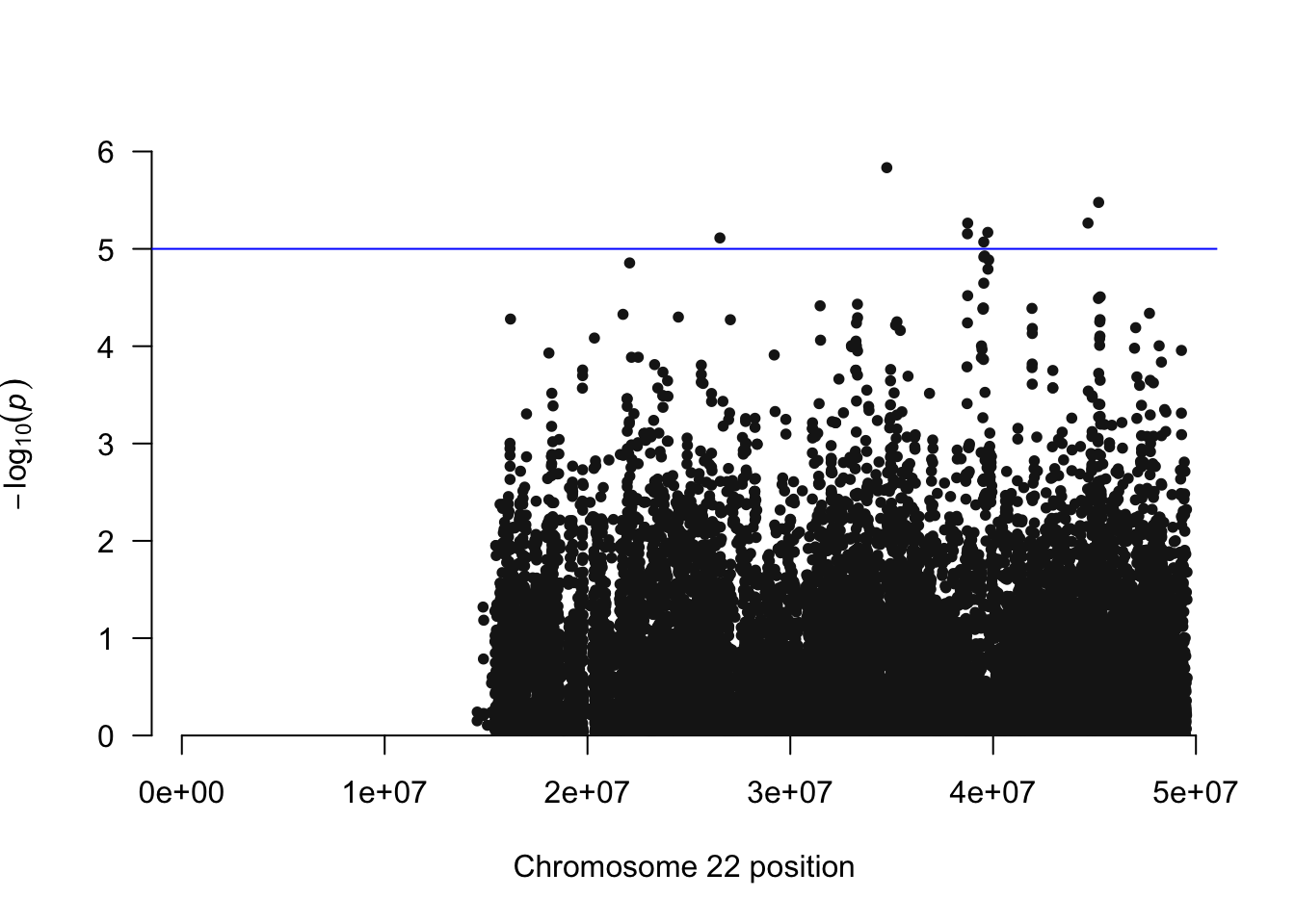

Past versions of “intrinsic growth phenotype GWAS-4.png”

Version	Author	Date
e73a329	Hae Kyung Im	2020-01-27

Simulate phenotype

set.seed(10) ## to get the same simulated values each time
simpheno = popinfo %>% mutate(pheno=rnorm(nrow(popinfo)))
write_tsv(simpheno, path=glue::glue("{work.dir}sim.pheno"))
## run association with plink
system(glue::glue("~/bin/plink --bfile {work.dir}hapmapch22 --linear --pheno {work.dir}sim.pheno --pheno-name pheno --maf 0.05 --out {work.dir}output/simpheno") )
simpheno.assoc = read.table(glue::glue("{work.dir}output/simpheno.assoc.linear"),header=T,as.is=T)
hist(simpheno.assoc$P)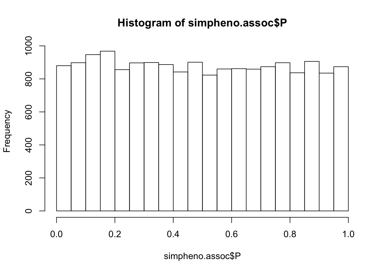

Past versions of “simulated phenotype-1.png”

Version	Author	Date
e73a329	Hae Kyung Im	2020-01-27

qqunif(simpheno.assoc$P)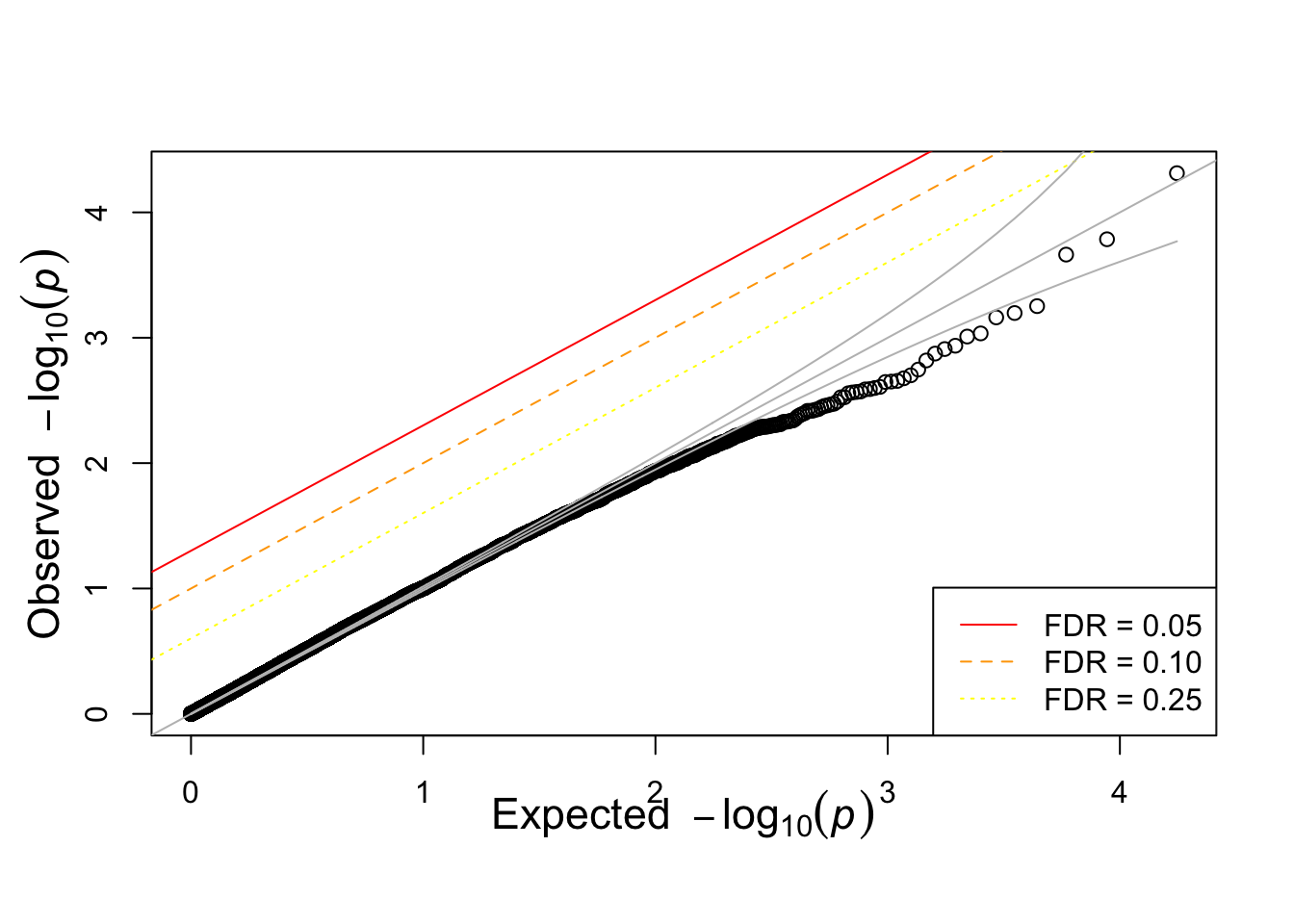

Past versions of “simulated phenotype-2.png”

Version	Author	Date
e73a329	Hae Kyung Im	2020-01-27

manhattan(simpheno.assoc, chr="CHR", bp="BP", snp="SNP", p="P" )

Past versions of “simulated phenotype-3.png”

Version	Author	Date
e73a329	Hae Kyung Im	2020-01-27

PCA calculation using plink

## generate PCs using plink
system(glue::glue("~/bin/plink --bfile {work.dir}hapmapch22 --pca --out {work.dir}output/pca"))
## read plink calculated PCs
pcplink = read.table(glue::glue("{work.dir}output/pca.eigenvec"),header=F, as.is=T)
names(pcplink) = c("FID","IID",paste0("PC", c(1:(ncol(pcplink)-2))) )
pcplink = popinfo %>% left_join(superpop,by=c("population"="Population")) %>% inner_join(pcplink, by=c("FID"="FID", "IID"="IID"))

## plot PC1 vs PC2
pcplink %>% ggplot(aes(PC1,PC2,col=population,shape=SuperPop)) + geom_point(size=3,alpha=.7) + theme_bw(base_size = 15)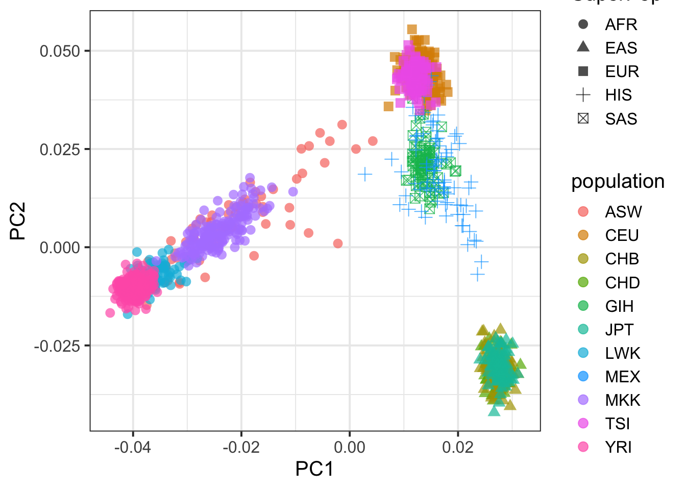

Past versions of “PCA calculation-1.png”

Version	Author	Date
e73a329	Hae Kyung Im	2020-01-27

manhattan(simpheno.assoc, chr="CHR", bp="BP", snp="SNP", p="P" ,main="Simulated Phenotype")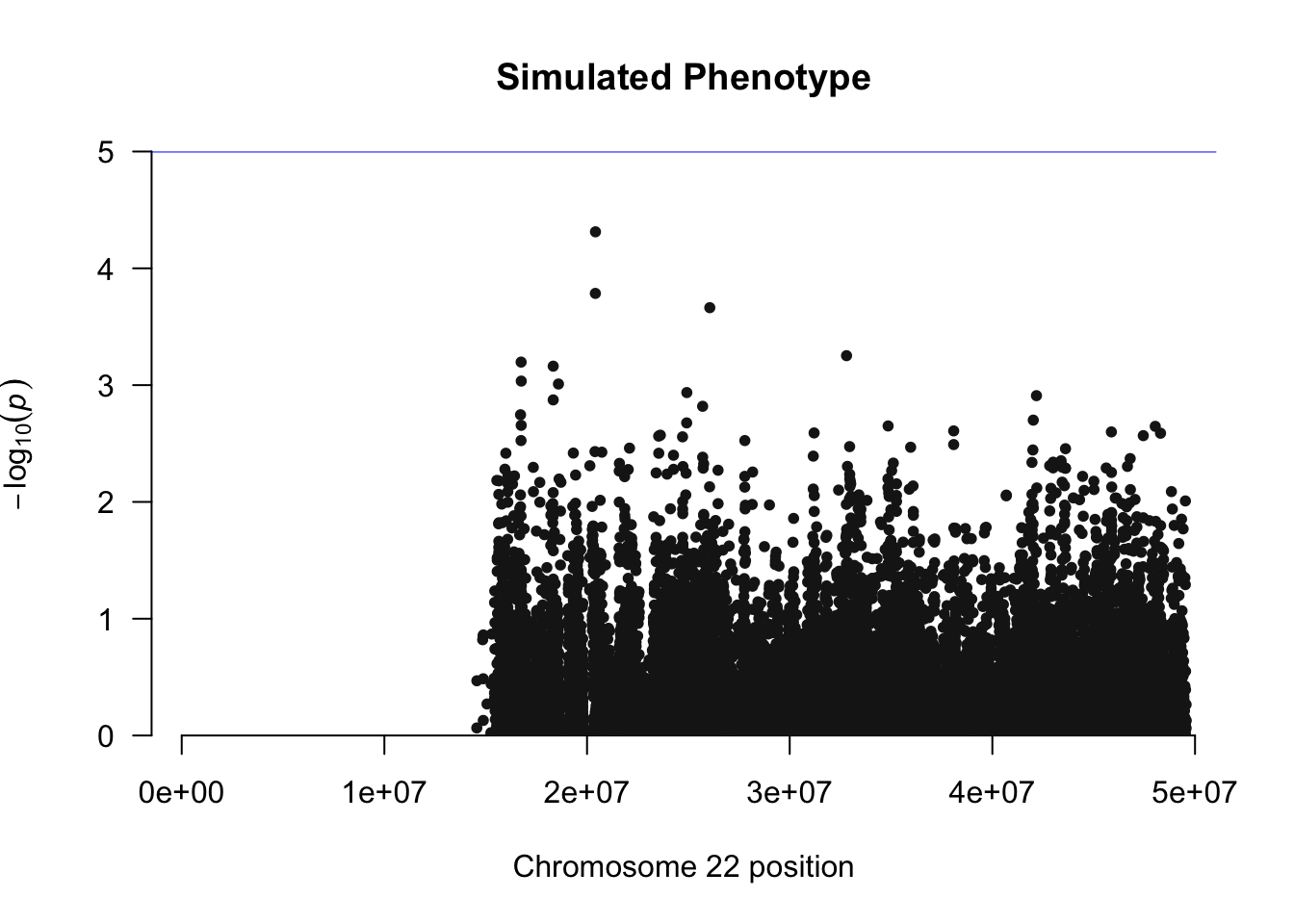

Past versions of “PCA calculation-2.png”

Version	Author	Date
e73a329	Hae Kyung Im	2020-01-27

runnig igrowth GWAS using PCs

system(glue::glue("~/bin/plink --bfile {work.dir}hapmapch22 --linear --pheno {work.dir}igrowth.pheno --pheno-name growth --covar {work.dir}output/pca.eigenvec --covar-number 1-4 --hide-covar --maf 0.05 --out {work.dir}output/igrowth-adjPC"))
igrowth.adjusted.assoc = read.table(glue::glue("{work.dir}output/igrowth-adjPC.assoc.linear"),header=T,as.is=T)
##indadd = igrowth.adjusted.assoc$TEST=="ADD"
titulo = "igrowh association adjusted for PCs"
hist(igrowth.adjusted.assoc$P,main=titulo)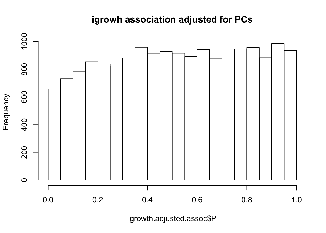

Past versions of “igrowth GWAS with PC-1.png”

Version	Author	Date
e73a329	Hae Kyung Im	2020-01-27

qqunif(igrowth.adjusted.assoc$P,main=titulo)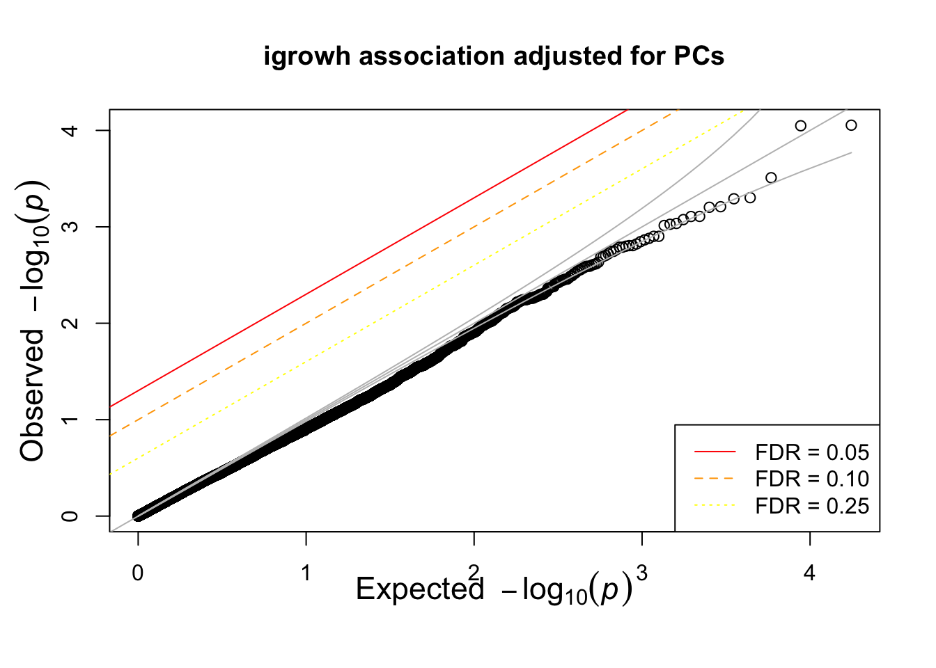

Past versions of “igrowth GWAS with PC-2.png”

Version	Author	Date
e73a329	Hae Kyung Im	2020-01-27

calculate Zscores

genomic.control = function(pvec)
{
 z = qnorm(pvec / 2)
 lambda = round(median(z^2) / 0.4549, 3)
 lambda
}

Session information

sessionInfo()

R version 3.6.1 (2019-07-05)
Platform: x86_64-apple-darwin15.6.0 (64-bit)
Running under: macOS Catalina 10.15.2

Matrix products: default
BLAS:   /Library/Frameworks/R.framework/Versions/3.6/Resources/lib/libRblas.0.dylib
LAPACK: /Library/Frameworks/R.framework/Versions/3.6/Resources/lib/libRlapack.dylib

locale:
[1] en_US.UTF-8/en_US.UTF-8/en_US.UTF-8/C/en_US.UTF-8/en_US.UTF-8

attached base packages:
[1] stats     graphics  grDevices utils     datasets  methods   base     

other attached packages:
 [1] qqman_0.1.4     forcats_0.4.0   stringr_1.4.0   dplyr_0.8.3    
 [5] purrr_0.3.3     readr_1.3.1     tidyr_1.0.0     tibble_2.1.3   
 [9] ggplot2_3.2.1   tidyverse_1.2.1

loaded via a namespace (and not attached):
 [1] tidyselect_0.2.5 xfun_0.11        haven_2.2.0      lattice_0.20-38 
 [5] colorspace_1.4-1 vctrs_0.2.0      generics_0.0.2   htmltools_0.4.0 
 [9] yaml_2.2.0       utf8_1.1.4       rlang_0.4.1      later_1.0.0     
[13] pillar_1.4.2     withr_2.1.2      glue_1.3.1       calibrate_1.7.5 
[17] modelr_0.1.5     readxl_1.3.1     lifecycle_0.1.0  munsell_0.5.0   
[21] gtable_0.3.0     workflowr_1.5.0  cellranger_1.1.0 rvest_0.3.5     
[25] evaluate_0.14    labeling_0.3     knitr_1.26       httpuv_1.5.2    
[29] curl_4.2         fansi_0.4.0      broom_0.5.2      Rcpp_1.0.3      
[33] promises_1.1.0   backports_1.1.5  scales_1.1.0     jsonlite_1.6    
[37] farver_2.0.1     fs_1.3.1         hms_0.5.2        digest_0.6.22   
[41] stringi_1.4.3    grid_3.6.1       rprojroot_1.3-2  cli_1.1.0       
[45] tools_3.6.1      magrittr_1.5     lazyeval_0.2.2   crayon_1.3.4    
[49] whisker_0.4      pkgconfig_2.0.3  zeallot_0.1.0    MASS_7.3-51.4   
[53] xml2_1.2.2       lubridate_1.7.4  assertthat_0.2.1 rmarkdown_1.17  
[57] httr_1.4.1       rstudioapi_0.10  R6_2.4.1         nlme_3.1-142    
[61] git2r_0.26.1     compiler_3.6.1