RatXcan Tutorial

Author

Sabrina Mi

Published

March 1, 2024

Data Requirements

genotype (plink bed/bim/fam format)
phenotype (TSV with columns FID, IID, phenotypes)
prediction weights (*.db models on https://predictdb.org)

All of the data and prediction models used in the tutorial can be downloaded from Box: https://uchicago.box.com/v/ratxcan-tutorial.

Software Requirements

plink
gcta
metaxcan (included in Box folder)
- set up conda environment

conda env create -f /Users/sabrinami/ratxcan-tutorial/MetaXcan/software/conda_env.yaml
conda activate imlabtools

Also check that the folders containing compiled plink and gcta binary files are in your $PATH variable.

Setup

In this section, we generate all results needed for the mixed effects modeling (predicted gene expression, genetic relatedness, and heritability)

Define Paths

PRE="/Users/sabrinami/ratxcan-tutorial" ## Replace with path to downloaded ratxcan-tutorial folder

OUTPUT="$PRE/output"

METAXCAN="$PRE/MetaXcan"
MODEL="$PRE/models"

GENO_PREFIX="$PRE/data/genotype/rat6k"

Both VCF and bed/bim/fam formatted genotypes are used, convert files if needed:

plink --bfile $GENO_PREFIX --recode vcf --out $GENO_PREFIX
gzip ${GENO_PREFIX}.vcf

Predict Expression

The models folder contains PrediXcan prediction models trained on 5 tissues:

nucleus accumbens (AC-filtered.db)
infralimbic cortex (IL-filtered.db)
lateral habenula (LH-filtered.db)
prelimbic cortex (PL-filtered.db)
orbitofrontal cortex (VO-filtered.db)

For the tutorial, we’ll use the AC model.

conda activate imlabtools
python ${METAXCAN}/software/Predict.py \
--model_db_path ${MODEL}/AC-filtered.db \
--model_db_snp_key rsid \
--vcf_genotypes ${GENO_PREFIX}.vcf.gz \
--vcf_mode genotyped \
--on_the_fly_mapping METADATA "{}_{}_{}_{}" \
--prediction_output $OUTPUT/AC-filtered-rat6k__predict.txt  \
--prediction_summary_output $OUTPUT/AC-filtered-rat6k__summary.txt \
--throw

Compute Genetic Relatedness and Heritability

GCTA outputs a genetic relatedness matrix (GRM), then computes heritability (h2) for a given phenotype data. The following example uses bodylength data.

## Compute GRM
gcta --bfile $GENO/rat6k --make-grm-bin --out $OUTPUT/rat6k
## Compute h2
## argument --mpheno specifies fam column to be used as phenotype, 1 for bodylength and 2 for bmi
gcta --grm $OUTPUT/rat6k --reml --pheno $PRE/data/phenotype/pheno.fam --mpheno 1 --out $OUTPUT/bodylen_h2

Heritability is estimated as V(G)/Vp Variance. In this case, we extract h2_bodylen = 0.390288 from the gcta results summary:

Summary result of REML analysis:
Source  Variance    SE
V(G)    0.395810    0.027842
V(e)    0.618337    0.014383
Vp  1.014147    0.027031
V(G)/Vp 0.390288    0.019209

Prepare Inputs for Mixed Effect Model

Setup

Load Libraries and Gist Functions:

## compare observed correlation with null correlation plotting functions
suppressMessages(devtools::source_gist("a925fea01b365a8c605e")) ## qqR fn https://gist.github.com/hakyim/a925fea01b365a8c605e
suppressMessages(devtools::source_gist("38431b74c6c0bf90c12f")) ## qqunif https://gist.github.com/hakyim/38431b74c6c0bf90c12f
## ratxcan functions
suppressMessages(devtools::source_gist("115403f16bec0a0e871f3616d552ce9b")) ## https://gist.github.com/hakyim/115403f16bec0a0e871f3616d552ce9b 

suppressMessages(library(tidyverse))
suppressMessages(library(glue))
suppressMessages(library(readr))
suppressMessages(library(biomaRt))

## to install qvalue
## if (!require("BiocManager", quietly = TRUE))
   ## install.packages("BiocManager")
## BiocManager::install("biomaRt")

Replace with your path to downloaded ratxcan-tutorial folder:

PRE <- "/Users/sabrinami/ratxcan-tutorial"
OUTPUT <- glue("{PRE}/output")

Read in GRM, h2, phenotypes, and predicted gene expression

## read grm
grm_mat <- read_GRMBin(glue("{OUTPUT}/rat6k.grm"))
grm_id <- read_tsv(glue("{OUTPUT}/rat6k.grm.id"), col_names = FALSE)

Rows: 5628 Columns: 2
── Column specification ────────────────────────────────────────────────────────
Delimiter: "\t"
chr (2): X1, X2

ℹ Use `spec()` to retrieve the full column specification for this data.
ℹ Specify the column types or set `show_col_types = FALSE` to quiet this message.

names(grm_id) <- c("FID","IID")
## read h2
tempo <- read_tsv(glue("{OUTPUT}/bodylen_h2.hsq")) %>% filter(Source=="V(G)/Vp")

Warning: One or more parsing issues, call `problems()` on your data frame for details,
e.g.:
  dat <- vroom(...)
  problems(dat)

Rows: 10 Columns: 3
── Column specification ────────────────────────────────────────────────────────
Delimiter: "\t"
chr (1): Source
dbl (2): Variance, SE

ℹ Use `spec()` to retrieve the full column specification for this data.
ℹ Specify the column types or set `show_col_types = FALSE` to quiet this message.

bodylen_h2 <- tempo %>% pull(Variance)
bodylen_se <- tempo %>% pull(SE)

## read phenotype
pheno_df <- read_tsv(glue("{PRE}/data/phenotype/pheno.fam"), col_names = FALSE)

Rows: 5401 Columns: 4
── Column specification ────────────────────────────────────────────────────────
Delimiter: "\t"
chr (2): X1, X2
dbl (2): X3, X4

ℹ Use `spec()` to retrieve the full column specification for this data.
ℹ Specify the column types or set `show_col_types = FALSE` to quiet this message.

names(pheno_df) <- c("FID","IID","bodylen","bmi")
## read predicted expression
pred_expr <- read_tsv(glue("{OUTPUT}/AC-filtered-rat6k__predict.txt")) %>% 
  dplyr::select(-FID) %>%  # Remove the FID column
  mutate(IID = str_split(IID, "_", simplify = TRUE)[, 1])  # Keep the first part of IID

Rows: 5628 Columns: 5881
── Column specification ────────────────────────────────────────────────────────
Delimiter: "\t"
chr    (2): FID, IID
dbl (5879): ENSRNOG00000015552, ENSRNOG00000016054, ENSRNOG00000049505, ENSR...

ℹ Use `spec()` to retrieve the full column specification for this data.
ℹ Specify the column types or set `show_col_types = FALSE` to quiet this message.

Summarize median predicted expression for all genes:

med_expr <- sapply(pred_expr %>% dplyr::select(-IID) %>% na.omit(), function(x) median(x, na.rm = TRUE)) %>% unname
summary(med_expr)

     Min.   1st Qu.    Median      Mean   3rd Qu.      Max. 
-4742.218    -0.442     0.000    -0.646     0.368  1998.544

Plot distribution of median gene expression with outliers removed:

lower <- quantile(med_expr, 0.01)
upper <- quantile(med_expr, 0.99)
filter_med_expr <- med_expr[med_expr >= lower & med_expr <= upper]
# breaks <- seq(min(med_expr), max(med_expr), by = 0.5)  # Adjust the 'by' value as needed
hist(filter_med_expr, main = "Med", xlab = "Values", ylab = "Frequency", col = "lightblue", border = "black")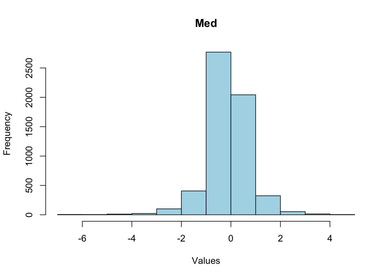

Final check that IIDs between phenotype and genotype matrices align:

idlist <- intersect(pheno_df$IID, grm_id$IID)
grm_mat <- grm_mat[idlist,idlist]
pheno_df <- pheno_df %>% filter(IID %in% idlist) 
if(!identical(colnames(grm_mat),pheno_df$IID))message("IIDs are not aligned between GRM and phenotype")

Convert to Matrices

ymat = matrix( pheno_df$bodylen, nrow(pheno_df),1 )
rownames(ymat) = pheno_df$IID

exp_mat = as.matrix(pred_expr %>% dplyr::select(-IID))
rownames(exp_mat) = pred_expr$IID
exp_mat = exp_mat[rownames(ymat),]
if(!identical(rownames(exp_mat), rownames(ymat))) warning("IDs not matched")

RatXcan Association

The end goal is to compute gene-level associations under the mixed effect model $Y = T b + u + \epsilon$, where

$Y$ is the phenotype
$T$ is predicted gene expression
$u$ is the random effect with covariance given by the genetic relatedness matrix ($GRM$)
$\epsilon$ is uncorrelated noise

The difference between RatXcan and PrediXcan is the $u$ term accounting for correlated effects due to relatedness. The $GRM$ and $h2$ estimates are needed to decorrelate the error term $u+\epsilon$, so that traditional linear regression can replace mixed modeling fitting.

Run regression

lmmGRM performs the decorrelation and linear regression. It takes phenotype, GRM, h2, and predicted expression as input, and computes gene-level correlation and p-value with and without correction accounting for relatedness.

## HERE WE USE THE FULL GRM MATRIX AND CALCULATE THE INVERSE OF THE SIGMA MATRIX}
## define lmm association function 
lmmGRM = function(pheno, grm_mat, h2, pred_expr, pheno_id_col=1,pheno_value_cols=6:6,out=NULL)
{
  ## input pheno is a data frame with id column pheno_id_col=1 by default
  ## phenotype values are in pheno_value_cols, 6:6 by default (SCORE column location in plink output), it can have more than one phenotype
  ## but h2 has to be the same, this is useful when running simulations with different h2
  ## call lmmXcan(pheno %>% select(IID,SCORE))
  
  ## format pheno to matrix form
  phenomat <- as.matrix(pheno[,pheno_value_cols])
  rownames(phenomat) <- pheno[[pheno_id_col]]
  
  ## turn pred_expr into matrix with rownames =IID, keep only IIDs in ymat
  exp_mat = as.matrix(pred_expr %>% dplyr::select(-IID))
  rownames(exp_mat) = pred_expr$IID

  ## align pheno and expr matrices
  idlist = intersect(rownames(phenomat), rownames(exp_mat))
  
  nsam = length(idlist)
  
    ## number
  num_genes <- ncol(exp_mat)

  print(glue("{nsam} samples, {num_genes} genes used in association test"))
  ## CALCULATE SIGMA
    ID_mat = diag(rep(1,nsam))
  
  Sigma = grm_mat[idlist,idlist] * h2 + (1 - h2) * ID_mat
  
  Sig_eigen = eigen(Sigma)
  rownames(Sig_eigen$vectors) = rownames(Sigma)
  
  isighalf = Sig_eigen$vectors %*% diag( 1 / sqrt(  Sig_eigen$values  ) ) %*% t(Sig_eigen$vectors)
  

  ## perform raw association
  cormat_raw = matrix_lm(phenomat[idlist,, drop = FALSE], exp_mat[idlist,])
  pmat_raw = cor2pval(cormat_raw,nsam)
  colnames(pmat_raw) <- gsub("cor_", "pval_", colnames(pmat_raw))
  
  ## perform corrected association
  cormat_correct = matrix_lm(isighalf%*% phenomat[idlist,, drop = FALSE], isighalf %*% exp_mat[idlist,])
  pmat_correct = cor2pval(cormat_correct,nsam)
  colnames(pmat_correct) <- gsub("cor_", "pval_", colnames(pmat_correct))
  
  # write outputs to file
  if(!is.null(out))
  {
    saveRDS(cormat_correct,file = glue("{out}_cormat_correct.RDS"))
    saveRDS(pmat_correct,  file = glue("{out}_pmat_correct.RDS"))
    saveRDS(cormat_raw,    file = glue("{out}_cormat_raw.RDS"))
    saveRDS(pmat_raw,      file = glue("{out}_pmat_raw.RDS"))
  }
  res = list(
    cormat_correct=cormat_correct, 
    pmat_correct=pmat_correct, 
    cormat_raw=cormat_raw, 
    pmat_raw=pmat_raw)
  return(res)
  
}

trait = "bodylen"
h2 = bodylen_h2
h2se = bodylen_h2+bodylen_se
##pheno, grm_mat, h2, pred_expr,pheno_id_col=1,pheno_value_cols=6:6,out=NULL

res_h2 <- lmmGRM(pheno_df,grm_mat, h2, pred_expr,pheno_id_col=1, pheno_value_cols=which(colnames(pheno_df)==trait))

5401 samples, 5879 genes used in association test

# png(glue("{OUTPUT}/bodylen-AC-lmmGRM.png"))qqunif.compare(res_h2$pmat_raw,res_h2$pmat_correct,main=glue("Ratxcan bodylength") )saveRDS(res_h2,glue("{OUTPUT}/bodylen_AC_h2.RDS"))

Plot P-values

The following QQ-plot shows the distribution of p-values of gene-trait associations: blue dots are the p-values with mixed effects correction and black dots are the inflated p-values.

#png(glue("{OUTPUT}/bodylen-AC-lmmGRM.png"))
qqunif.compare(res_h2$pmat_raw,res_h2$pmat_correct,main=glue("RatXcan bodylength") )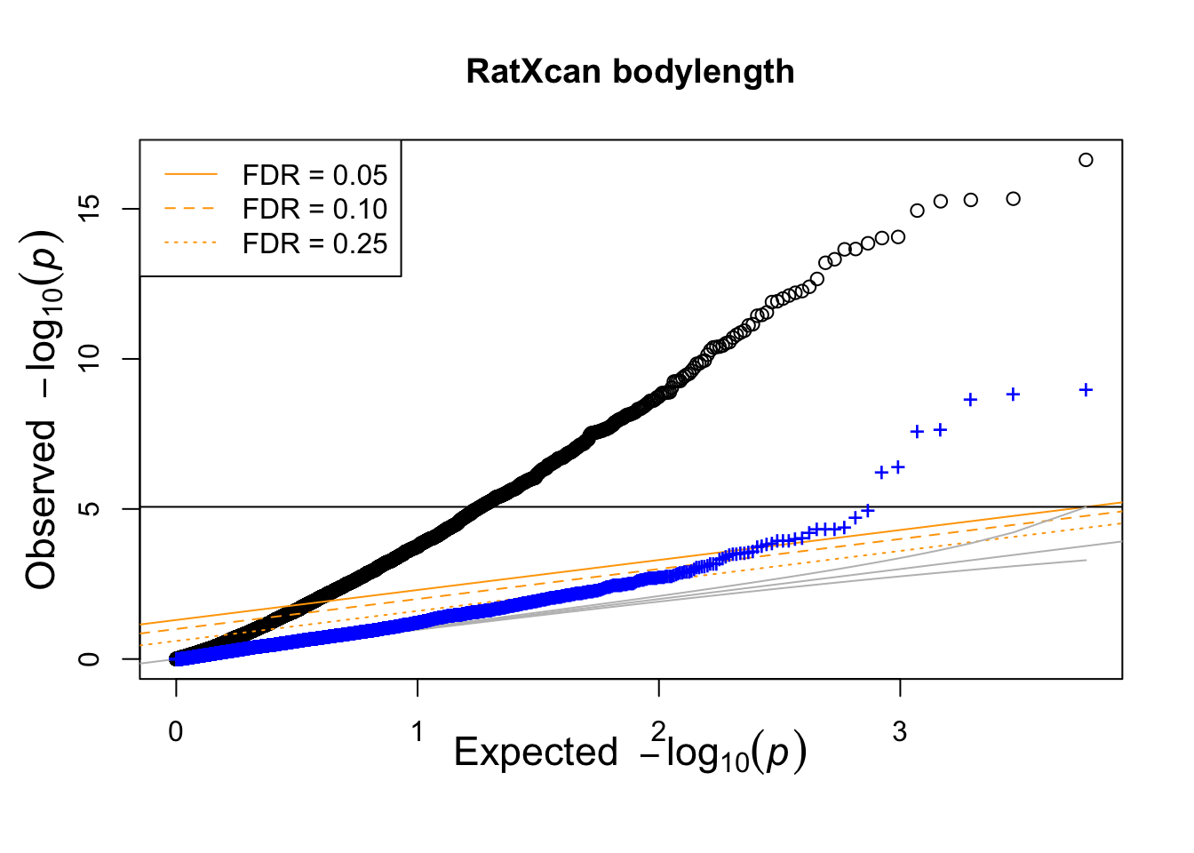

The following Manhattan plot was generated with Natasha Santhanam’s function:

## here
## qq_manhattan(tempo %>% rename(pvalue=p_acat_6))
library(ggrepel)
gg_manhattan <- function(df, titulo="",significance_threshold = 0.05) {
  ## USAGE: gg_manhattan(df,0.05)
  ## df has columns: pvalue, chr (numeric), and start (position)
  ## significance threshold gets divided by the number of tests
  ## 
  df <- df %>% filter(!is.na(pvalue))
  # Calculate cumulative base pair positions
  data_cum <- df %>%
    group_by(chr) %>%
    summarise(max_bp = as.numeric(max(start)), .groups = 'drop') %>%
    mutate(bp_add = lag(cumsum(max_bp), default = 0))

  gwas_data <- df %>%
    inner_join(data_cum, by = "chr") %>%
    mutate(bp_cum = start + bp_add)

  # Calculate axis labels
  axis_set <- gwas_data %>%
    group_by(chr) %>%
    summarize(center = mean(bp_cum), .groups = 'drop')

  # Determine the ylim based on the most significant p-value
  ylim <- gwas_data %>%
    filter(pvalue == min(pvalue)) %>%
    summarise(ylim = abs(floor(log10(pvalue))) + 2) %>%
    pull(ylim)

  # Calculate the genome-wide significance level
  sig <- significance_threshold / nrow(df)

  # Construct the Manhattan plot
  manhattan_plot <- ggplot(gwas_data, aes(x = bp_cum, y = -log10(pvalue), color = as.factor(chr), size = -log10(pvalue))) +
    geom_hline(yintercept = -log10(sig), color = "grey40", linetype = "dashed") +
    geom_hline(yintercept = -log10(0.0001), color = "red", linetype = "dashed") +
    geom_point(alpha = 0.75, shape = 19) + # Simplified shape decision for clarity
    geom_label_repel(aes(label = ifelse(pvalue <= sig, gene_name, "")), size = 3) +
    ylim(c(0, ylim)) +
    scale_x_continuous(labels = axis_set$chr, breaks = axis_set$center) +
    scale_color_manual(values = rep(c("dodgerblue4", "midnightblue"), length(unique(axis_set$chr)))) +
    scale_size_continuous(range = c(0.5, 3)) +
    labs(x = NULL, y = expression(-log[10](italic(p)))) +
    theme_minimal() +
    theme(legend.position = "none",
          panel.border = element_blank(),
          panel.grid.major.x = element_blank(),
          panel.grid.minor.x = element_blank(),
          axis.text.x = element_text(angle = 90, size = 12),
          axis.text.y = element_text(size = 12, vjust = 0),
          axis.title = element_text(size = 20))

  if(titulo !="") manhattan_plot = manhattan_plot + ggtitle(titulo)
  return(manhattan_plot)
}

We used biomaRt to annotate genes:

human = biomaRt::useEnsembl(biomart='ensembl', dataset="hsapiens_gene_ensembl", mirror = "useast")

Ensembl site unresponsive, trying asia mirror

Ensembl site unresponsive, trying www mirror

attributes = c("ensembl_gene_id", "external_gene_name", "rnorvegicus_homolog_ensembl_gene", "rnorvegicus_homolog_associated_gene_name")
orth.rats = biomaRt::getBM(attributes, filters="with_rnorvegicus_homolog",values=TRUE, mart = human, uniqueRows=TRUE)
# saveRDS(orth.rats,file=glue("{PRE}/data/expression/orth.rats.RDS"))

bodylen_res <- read_csv(glue("{PRE}/data/ratxcan-bodylen-results.csv")) %>% dplyr::select(gene_name, AC, chr, start) %>% rename(pvalue=AC)

Rows: 10933 Columns: 17
── Column specification ────────────────────────────────────────────────────────
Delimiter: ","
chr  (5): gene_name, hugo_gene, trait, gene, gene_id
dbl (12): p_acat_6, chr, start, qval, p_human, BR, AC, IL, LH, PL, VO, p_acat_5

ℹ Use `spec()` to retrieve the full column specification for this data.
ℹ Specify the column types or set `show_col_types = FALSE` to quiet this message.

gg <- gg_manhattan(bodylen_res, titulo="RatXcan Bodylength (AC tissue)")
# ggsave(glue("{OUTPUT}/bodylen-manhattan-p_AC.png"))
print(gg)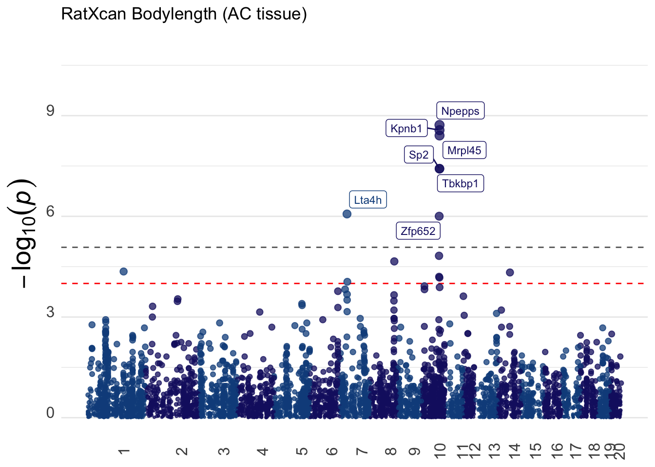

The full RatXcan results includes tissue-specific p-values (AC, IL, LH, PL, VO) and a combination p-value (ACAT), as well as PhenomeXcan results for corresponding human phenotypes and genes. The datasets are included in the data subdirectory and accessible on https://imlab.shinyapps.io/RatXcan/.